Perform Max-P regionalization to maximize the number of spatially contiguous regions such that each region satisfies a minimum threshold constraint on a specified attribute. This is useful for creating regions that meet minimum population or sample size requirements.
Usage
max_p_regions(
  data,
  attrs = NULL,
  threshold_var,
  threshold,
  weights = "queen",
  bridge_islands = FALSE,
  compact = FALSE,
  compact_weight = 0.5,
  compact_metric = "centroid",
  homogeneous = TRUE,
  n_iterations = 100L,
  n_sa_iterations = 100L,
  cooling_rate = 0.99,
  tabu_length = 10L,
  scale = TRUE,
  seed = NULL,
  verbose = FALSE
)
Arguments
- data
An sf object with polygon or point geometries.
- attrs
Character vector of column names to use for computing within-region dissimilarity (e.g.,
c("var1", "var2")). If NULL, uses all numeric columns.- threshold_var
Character. Name of the column containing the threshold variable (e.g., population, income). Each region must have a sum of this variable >=
threshold.- threshold
Numeric. Minimum sum of
threshold_varrequired per region.- weights
Spatial weights specification. Can be:
"queen"(default): Polygons sharing any boundary point are neighbors"rook": Polygons sharing an edge are neighborsAn
nbobject from spdep or created withsp_weights()A list for other weight types:
list(type = "knn", k = 6)for k-nearest neighbors, orlist(type = "distance", d = 5000)for distance-based weights
KNN weights guarantee connectivity (no islands), which can be useful for datasets with disconnected polygons.
- bridge_islands
Logical. If TRUE, automatically connect disconnected components (e.g., islands) using nearest-neighbor edges. If FALSE (default), the function will error when the spatial weights graph is disconnected. This is useful for datasets like LA County with Catalina Islands, or archipelago data where physical adjacency doesn't exist but regionalization is still desired.
- compact
Logical. If TRUE, optimize for region compactness in addition to attribute homogeneity. Compact regions have more regular shapes, which is useful for sales territories, patrol areas, and electoral districts. Default is FALSE.
- compact_weight
Numeric between 0 and 1. Weight for compactness vs attribute homogeneity when
compact = TRUE. Higher values prioritize compact shapes over attribute similarity. Default is 0.5.- compact_metric
Either "centroid" (the default) or "nmi" (Normalized Moment of Inertia).
- homogeneous
Logical. If TRUE, minimizes within-region dissimilarity, so that regions are internally homogeneous. If FALSE, maximizes within-region dissimilarity.
- n_iterations
Integer. Number of construction phase iterations (default 100). Higher values explore more random starting solutions.
- n_sa_iterations
Integer. Number of simulated annealing iterations (default 100). Set to 0 to skip the SA refinement phase.
- cooling_rate
Numeric. SA cooling rate between 0 and 1 (default 0.99). Smaller values cool faster, larger values allow more exploration.
- tabu_length
Integer. Length of tabu list for SA phase (default 10).
- scale
Logical. If TRUE (default), standardize attributes before computing dissimilarity.
- seed
Optional integer for reproducibility.
- verbose
Logical. Print progress messages.
Value
An sf object with a .region column containing region assignments.
Metadata is stored in the "spopt" attribute, including:
algorithm: "max_p"
n_regions: Number of regions created (the "p" in max-p)
objective: Total within-region sum of squared deviations
threshold_var: Name of threshold variable
threshold: Threshold value used
solve_time: Time to solve in seconds
mean_compactness: Mean Polsby-Popper compactness (if
compact = TRUE)region_compactness: Per-region compactness scores (if
compact = TRUE)
Details
The Max-P algorithm (Duque, Anselin & Rey, 2012; Wei, Rey & Knaap, 2021) solves the problem of aggregating n geographic areas into the maximum number of homogeneous regions while ensuring:
Each region is spatially contiguous (connected)
Each region satisfies a minimum threshold on a specified attribute
The algorithm has two phases:
Construction phase: Builds feasible solutions via randomized greedy region growing. Multiple random starts are explored in parallel.
Simulated annealing phase: Refines solutions by moving border areas between regions to minimize within-region dissimilarity while respecting constraints.
When compact = TRUE, the algorithm additionally optimizes for compact region
shapes based on Feng, Rey, & Wei (2022). Compact regions:
Minimize travel time within regions (useful for service territories)
Reduce gerrymandering potential (electoral districts)
Often result in finding MORE regions due to efficient space usage
Compactness metric: This implementation provides two options for the compactness metric used during optimization. The Normalized Moment of Inertia (NMI) described in Feng et al. (2022) can be used. However, the default option is a dispersion measure. The dispersion measure has two advantages:
Point-based regionalization: The algorithm works with both polygon and point geometries. For point data, use KNN or distance-based weights (e.g.,
weights = list(type = "knn", k = 6)).Computational efficiency: Centroid dispersion is O(n) per region versus O(v) for NMI where v = total polygon vertices.
For polygon data, centroids are computed via sf::st_centroid(). Users should
be aware that centroid-based compactness may be less accurate for highly
irregular shapes or large, sparsely-populated areas where the centroid poorly
represents the polygon's spatial extent.
The reported mean_compactness and region_compactness in results use
Polsby-Popper (4piA/P^2), a standard geometric compactness measure for
polygons. For point data, these metrics are not computed.
This implementation is optimized for speed using:
Parallel construction with early termination
Efficient articulation point detection for move eligibility
Incremental threshold tracking
References
Duque, J. C., Anselin, L., & Rey, S. J. (2012). The max-p-regions problem. Journal of Regional Science, 52(3), 397-419.
Wei, R., Rey, S., & Knaap, E. (2021). Efficient regionalization for spatially explicit neighborhood delineation. International Journal of Geographical Information Science, 35(1), 135-151. doi:10.1080/13658816.2020.1759806
Feng, X., Rey, S., & Wei, R. (2022). The max-p-compact-regions problem. Transactions in GIS, 26, 717-734. doi:10.1111/tgis.12874
Examples
# \donttest{
library(sf)
nc <- st_read(system.file("shape/nc.shp", package = "sf"))
#> Reading layer `nc' from data source
#> `/Users/kylewalker/Library/R/arm64/4.5/library/sf/shape/nc.shp'
#> using driver `ESRI Shapefile'
#> Simple feature collection with 100 features and 14 fields
#> Geometry type: MULTIPOLYGON
#> Dimension: XY
#> Bounding box: xmin: -84.32385 ymin: 33.88199 xmax: -75.45698 ymax: 36.58965
#> Geodetic CRS: NAD27
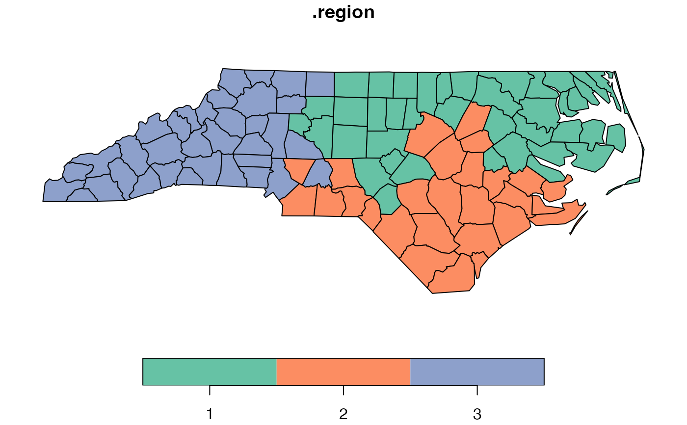
# Create regions where each has at least 100,000 in BIR74
result <- max_p_regions(
nc,
attrs = c("SID74", "SID79"),
threshold_var = "BIR74",
threshold = 100000
)
# Check number of regions created
attr(result, "spopt")$n_regions
#> [1] 3
# With compactness optimization (for sales territories)
result_compact <- max_p_regions(
nc,
attrs = c("SID74", "SID79"),
threshold_var = "BIR74",
threshold = 100000,
compact = TRUE,
compact_weight = 0.5
)
# Check compactness
attr(result_compact, "spopt")$mean_compactness
#> [1] 0.1982033
# Plot results
plot(result[".region"])
 # Point-based regionalization (e.g., store locations, sensor networks)
# Use KNN weights since points don't have polygon contiguity
points <- st_as_sf(data.frame(
x = runif(200), y = runif(200),
customers = rpois(200, 100),
avg_income = rnorm(200, 50000, 15000)
), coords = c("x", "y"))
result_points <- max_p_regions(
points,
attrs = "avg_income",
threshold_var = "customers",
threshold = 500,
weights = list(type = "knn", k = 6),
compact = TRUE
)
#> Error: max_p_regions: graph has 2 disconnected components.
#> Set `bridge_islands = TRUE` to automatically connect them using nearest-neighbor edges,
#> or provide a connected weights object (e.g., KNN weights).
# }
# Point-based regionalization (e.g., store locations, sensor networks)
# Use KNN weights since points don't have polygon contiguity
points <- st_as_sf(data.frame(
x = runif(200), y = runif(200),
customers = rpois(200, 100),
avg_income = rnorm(200, 50000, 15000)
), coords = c("x", "y"))
result_points <- max_p_regions(
points,
attrs = "avg_income",
threshold_var = "customers",
threshold = 500,
weights = list(type = "knn", k = 6),
compact = TRUE
)
#> Error: max_p_regions: graph has 2 disconnected components.
#> Set `bridge_islands = TRUE` to automatically connect them using nearest-neighbor edges,
#> or provide a connected weights object (e.g., KNN weights).
# }