library(tidycensus)
library(tidyverse)

top100metros <- get_acs(
  geography = "cbsa",
  variables = "B01003_001",
  year = 2022,
  survey = "acs1",
  geometry = TRUE
) %>%
slice_max(estimate, n = 100)Iterative ‘mapping’ in R
r
gis
data science
census
My book Analyzing US Census Data: Methods, Maps, and Models in R, published last year, covers a lot of the data science tips and tricks I’ve learned over the years. In my academic and consulting work, I apply a lot of additional workflows that the book doesn’t cover. This year on the blog, I’d like to share some brief examples of workflows I’ve found useful with a focus on applications to Census and demographic data.
In my consulting work, I’m commonly asked to build out maps, charts, or reports for a large number of cities or regions at once. The goal here is often to allow for rapid exploration / iteration, so a basic map template might be fine. Doing this for a few cities one-by-one isn’t a problem, but it quickly gets tedious when you have dozens, if not hundreds, of visuals to produce – and keeping all the results organized can be a pain.
Let’s tackle a hypothetical example. Your boss has assigned you the following task:
I’d like to look at geographic patterns in working from home for the 100 largest metro areas in the US.
At first, this may seem like a fairly significant research task. You need to do the following:
- Generate a list of the 100 largest metro areas by population in the US;
- Get data on working from home at a sufficiently granular geographic level to show patterns;
- Identify those geographies by metropolitan area, and subset appropriately;
- Make and deliver 100 maps.
This might seem like a lot of work, but it really isn’t too bad if you handle it the right way with R.
Getting demographic data with tidycensus
We’ll first need to identify the 100 largest metro areas in the US; fortunately, this is straightforward to accomplish with the tidycensus R package.
We’ve pulled data here from the 2022 1-year American Community Survey for core-based statistical areas (CBSAs), which includes metropolitan statistical areas. slice_max() gets us the 100 largest values of the estimate column, which in this case stores values on total population in 2022.
Next, we’ll need to grab data on the work-from-home share by Census tract, a reasonably granular Census geography with approximately 4,000 residents on average. Census tracts aren’t directly identifiable by metro, so we’ll get data for the entire US. With tidycensus, grabbing demographic data for all 50 US states + DC and Puerto Rico is straightforward; pass an appropriate vector to the state parameter as an argument.
us_wfh_tract <- get_acs(
  geography = "tract",
  variables = "DP03_0024P",
  state = c(state.abb, "DC", "PR"),
  year = 2022,
  geometry = TRUE
)

us_wfh_tract
Simple feature collection with 85396 features and 5 fields (with 337 geometries empty)
Geometry type: MULTIPOLYGON
Dimension: XY
Bounding box: xmin: -179.1467 ymin: 17.88328 xmax: 179.7785 ymax: 71.38782
Geodetic CRS: NAD83
# A tibble: 85,396 × 6
GEOID NAME variable estimate moe geometry
<chr> <chr> <chr> <dbl> <dbl> <MULTIPOLYGON [°]>
1 01089003100 Census Tract 3… DP03_00… 16 5.9 (((-86.59838 34.74091, -…
2 01089000501 Census Tract 5… DP03_00… 3.2 3.2 (((-86.65703 34.77881, -…
3 01089011021 Census Tract 1… DP03_00… 11.2 6.4 (((-86.78678 34.67045, -…
4 01095031200 Census Tract 3… DP03_00… 3.6 3.6 (((-86.17402 34.23036, -…
5 01073012401 Census Tract 1… DP03_00… 4.9 6.8 (((-86.90739 33.57447, -…
6 01073000800 Census Tract 8… DP03_00… 8.4 8.8 (((-86.86691 33.53711, -…
7 01073010402 Census Tract 1… DP03_00… 2.7 2.7 (((-86.99094 33.37425, -…
8 01073003900 Census Tract 3… DP03_00… 3.1 4.3 (((-86.87669 33.49688, -…
9 01073005908 Census Tract 5… DP03_00… 3.8 4.3 (((-86.689 33.60838, -86…
10 01103000100 Census Tract 1… DP03_00… 0 2.1 (((-86.97709 34.60967, -…
# ℹ 85,386 more rowsAs you can see above, we’ve fetched data on the share of the workforce working from home for all Census tracts in the United States.
Iterative spatial overlay
Our next step is to determine which of these Census tracts fall within each of the top 100 metro areas in the US. One way to accomplish this is with a spatial join; I’m going to show you an alternative workflow that I’ll call “iterative spatial overlay” which I like to use to organize my data.
I’m a huge fan of R’s list data structure to help with these tasks. I struggled with lists in R when I was first learning the language, but I now find lists essential. Lists are flexible data structures that can basically store whatever objects you want. I’m partial to the named list, in which those objects are accessible by name.
The code below is a simplified version of a workflow I commonly use. The split() command will split the top100metros object into a list of metro areas, organized by the name of the metro. We then iterate over this list with map(), doing a series of spatial analysis operations for each metro. In this case, I’m identifying which tracts fall within each metro area, first performing a spatial filter on tract points then filtering on those tract IDs. This helps circumvent any topology issues with polygon-on-polygon overlay.
One note - as I’m using formula notation with map(), each respective object in the list will be represented by .x as map() iterates over my list.
library(sf)
sf_use_s2(FALSE)

tract_points <- us_wfh_tract %>%
  st_point_on_surface()

us_wfh_metro <- top100metros %>%
  split(~NAME) %>%
  map(~{
    tract_ids <- tract_points %>%
      st_filter(.x) %>%
      pull(GEOID)

    us_wfh_tract %>%
      filter(GEOID %in% tract_ids)
  })
We now have the results of every operation organized by the metro area’s name. In RStudio, type us_wfh_metro followed by the $ sign, then use the Tab key to browse through the various metro areas.
us_wfh_metro$`Minneapolis-St. Paul-Bloomington, MN-WI Metro Area`Simple feature collection with 892 features and 5 fields
Geometry type: MULTIPOLYGON
Dimension: XY
Bounding box: xmin: -94.26152 ymin: 44.19584 xmax: -92.13481 ymax: 46.24697
Geodetic CRS: NAD83
# A tibble: 892 × 6
GEOID NAME variable estimate moe geometry
* <chr> <chr> <chr> <dbl> <dbl> <MULTIPOLYGON [°]>
1 27053021505 Census Tract 2… DP03_00… 11.8 4 (((-93.40064 45.01667, -…
2 27053026713 Census Tract 2… DP03_00… 18.2 4.5 (((-93.43159 45.0667, -9…
3 27053000102 Census Tract 1… DP03_00… 15.3 6.8 (((-93.29919 45.05114, -…
4 27053108700 Census Tract 1… DP03_00… 30.4 8.5 (((-93.24235 44.94837, -…
5 27053102100 Census Tract 1… DP03_00… 4.3 2.9 (((-93.3082 45.00603, -9…
6 27053026814 Census Tract 2… DP03_00… 4.1 2.4 (((-93.3211 45.10899, -9…
7 27053023802 Census Tract 2… DP03_00… 25.4 6.3 (((-93.32898 44.88885, -…
8 27053100800 Census Tract 1… DP03_00… 21.2 13.3 (((-93.30833 45.02409, -…
9 27053125800 Census Tract 1… DP03_00… 7.5 5.1 (((-93.26259 44.95375, -…
10 27053025403 Census Tract 2… DP03_00… 12.2 5.4 (((-93.28698 44.83271, -…
# ℹ 882 more rowsUsing map() to make… maps
One of the things I really like about list data structures is that I can use the map() family of functions in the purrr package (or lapply() if you prefer base R) to visualized my data and return those visualizations in the same organized format. Here, I’ll use map() to make 100 maps - one for each metro area.
library(mapview)
library(leaflet)

wfh_maps <- map(us_wfh_metro, ~{
  mapview(
    .x,
    zcol = "estimate",
    layer.name = "% working from home"
  )
})
As before, I can access each interactive map by name! This is often how I’ll keep my data organized and explore the various maps as needed.
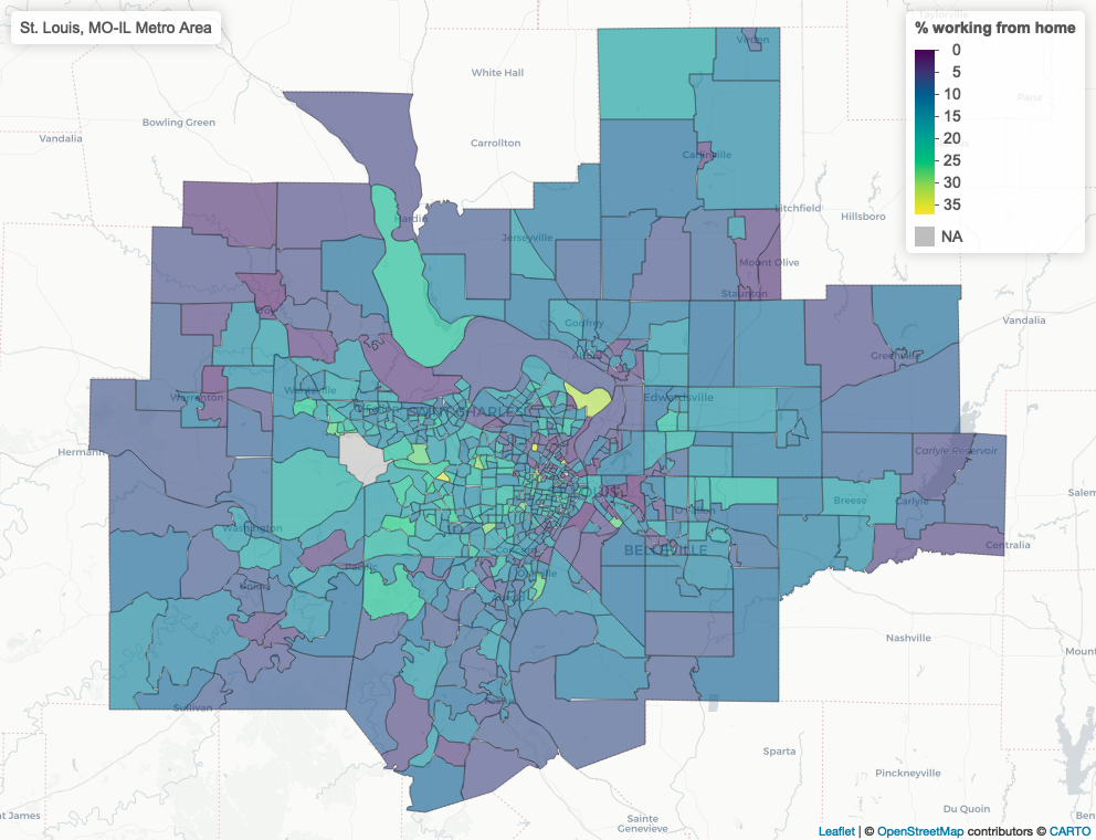
wfh_maps$`Dallas-Fort Worth-Arlington, TX Metro Area`Finally, I can also readily write out my maps to static screenshots using a similar workflow. In this case I’ll use an indexed walk() to step over each interactive map and write it to a static file with mapshot(). Note that the iwalk() function gives me access to .x, which is the list element (the map itself), and .y, which is the index - a character string representing the metro area’s name in this instance. I can use .y as the name of the file as well as the title of the map which will be added to the output.
library(glue)

iwalk(wfh_maps, ~{
  out_file <- glue("img/{.y}.png")

  .x@map %>%
    addControl(.y) %>%
    mapshot(file = out_file)
})
I now have 100 static maps in my img folder! They won’t be uniquely customized for each metro, but when time is of the essence, this workflow is often “good enough.”