If you follow me on any of my social media channels you’ve likely seen some of my “mapping millions of data points” posts. A few of these examples have covered statewide parcel data. In the industries where I consult - energy/land and real estate - parcel data is immensely valuable for understanding land ownership, right-of-way, valuation, and more. There are a tons of challenges in working with parcel data, however. High-quality parcel data can be expensive or difficult to access - and even if you get it, you’re dealing with huge files that are challenging to visualize and explore.
In this post, I’ll show you how I do it.
Getting parcel data for Texas
The public availability of parcel GIS data differs widely by state and by county. Some states, like Texas and Florida, consolidate and distribute parcel data from counties at the state level and make state-wide datasets available. Texas is a great example to work with, as the Texas Geographic Information Office makes a 2025 statewide parcel dataset available for bulk download. 253 of the state’s 254 counties are represented; only Donley County is missing.
Unzipping gets us an Esri file geodatabase a little over 7 GB in size. This is a hefty spatial dataset to work with, and file geodatabases are typically meant for use with commercial GIS software. If that’s not available to you, you’ll want to use tools for free and file formats that are more transparent. I’ll be using R and DuckDB via the duckspatial package; let’s get set up.
With duckspatial, we can use DuckDB’s spatial extension to read in our 7 GB file geodatabase lazily and inspect the data quickly.
There are 38 columns in the dataset that TxGIO has standardized across Texas’s counties. Our first few rows are from Travis County (Austin); we can see that some of the columns are populated, but others are not (e.g. year built is missing for these records), so we aren’t likely to have complete coverage for each column across the state.
While DuckDB can read from a file geodatabase directly, let’s get our parcel data into a DuckDB database before proceeding any further.
For a normal spatial dataset, we’d likely spin up a quick interactive map in R to explore our data. In my mapgl package, the mapboxgl_view() and maplibre_view() functions are great for this purpose. For a 14.3 million row, multi-gigabyte dataset, this simply won’t work, as it’ll overload your web browser (or possibly even your GIS software) quickly.
Aside from the size issue, there are several other challenges we’ll need to think through before visualizing our data. A few:
Column completeness. I mentioned this earlier; public statewide parcel data will likely have inconsistent or incomplete columns. If you try to map data with considerable missingness, it won’t be informative or will just look bad.
Polygon size. Parcels are typically very small. On an interactive map, it makes little sense to show parcels when zoomed out, as you can’t actually see most of them, especially within cities. So you’ll want to figure out a zoom-dependent strategy to handle this.
Parcel stacking. It’s common for parcel record datasets to include “stacked”, or repeated, geometries, as single parcels often include multiple records (e.g., a condominium complex with multiple owners). This can introduce confusing visual artifacts and obscured data.
Resolving all of this will require some decision-making around both data cleaning and data formats for visualization. We’ll first take a look at our data and see what we can reasonably represent statewide, and come up with a strategy for the parcel stacking issue.
Exploring columns in our data
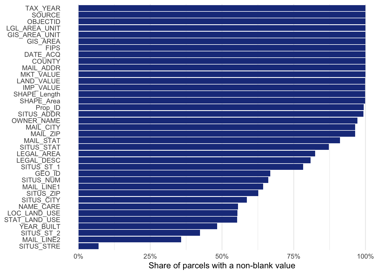
Let’s examine column completeness to start with, and see what we might be able to visualize. Most missing data in the dataset (as we saw above) is a blank string, not NA, so we’ll evaluate accordingly.
library(scales)parcels <-ddbs_open_dataset("~/data/tx_parcels.duckdb", layer ="tx_parcels")completeness <- parcels |>ddbs_drop_geometry() |>summarize(across(everything(),~mean(as.numeric(!is.na(.x) &trimws(as.character(.x)) !=""), na.rm =TRUE) )) |>collect() |>pivot_longer(everything(), names_to ="column", values_to ="share_filled")ggplot(completeness, aes(x = share_filled, y =reorder(column, share_filled))) +geom_col(fill ="#1e3a8a") +scale_x_continuous(labels =label_percent()) +labs(x ="Share of parcels with a non-blank value", y =NULL) +theme_minimal(base_size =11) +theme(panel.grid.major.y =element_blank())
Some columns are clear no-gos for statewide analysis; for example, we only have a little over 50% coverage for year built and land use. Ownership is mostly complete, as are the value columns (market, land, and improvement). However, this can be misleading. Let’s take a closer look at the value columns:
20 percent of the market value, 30 percent of the land value, and 56 percent of the improvement value columns are zero! So if we tried to visualize any of these columns, we’d be dealing with substantial coverage gaps. Beyond this, though, the zero-values likely mean substantively different things. A “0” improvement value may actually be meaningful, as vacant land won’t have improvements on it. However, in many cases, the “0” is also representing missing data here. So we have to proceed with caution, and really shouldn’t visualize the data statewide.
So we need to figure out what we can show. Ownership is often one of the most interesting parcel characteristics for energy / land / real estate clients. A compelling map might be a visualization of non-Texas ownership; specifically parcels where the listed owner is either in another state or international. Let’s take a quick look:
Around 11.7 million parcels list an owner in Texas; another 1.27 million are blank (though most of these are in Tarrant County, where “TX” is appended to the city in the data); and another 620,000 list “TEXAS”. Other states are well-represented, notably over 150k in California.
This does suggest an interesting map idea: the geography of out-of-state owners. We’ll come back to this when it’s time to prep the data for visualization.
Dealing with parcel stacking
Our next data wrangling step is handling the parcel stacking issue - duplicate geometries in our data that represent separate parcel records. Let’s first diagnose the issue. The geometry column is named SHAPE in this dataset, so we can use that as a unique identifier in our diagnosis.
Of the 14.3 million parcel records, we have around 13.5 million unique shapes. Around 932,000 records are in stacked parcels; the largest stack has over 11,300 records! Let’s take a look at the biggest stacks:
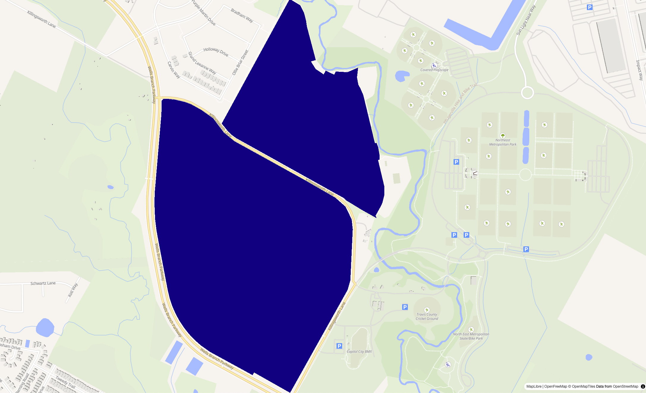
The biggest “stack” actually represents all parcel records that don’t have geometry. The other example - a parcel with 1210 records and 1083 owners - is a manufactured home community in Pflugerville, outside Austin. Each of the records represents a single mobile-home space but they all share the same parcel. For example:
We first do some wrangling inside the database to identify Texas and non-Texas owners, and clean up areas where we have data missingness (e.g. converting true blanks to NA in the address column).
We’ll then summarize twice over parcels grouped by their geometry and property ID. The first summarize collapses ownership records into tax accounts; the second collapses tax accounts into specific parcel geometries, collecting metadata along the way.
Handling owner information without losing anything is tricky, as we’ll in some cases have to condense 100s of owners into a single row of our dataset. We’ll do a couple things here: create an owners_all column that handles all of the owners, then an owner_names column that shows the first few owners in a multi-owner parcel.
Given that we grouped by the SHAPE column (the warning message we get), as_duckspatial_df() reconstructs the geometry for us, which we’ll need in the next step.
Preparing the data for visualization with freestiler
We’ve handled column inspection and wrangled our data. Now, we’ll need to iron out the visualization issues. Even though we’ve cleaned up the stacked geometry, we still have 13.5 million unique polygons to visualize… which is way too many to load directly into a modern web map.
The solution is to convert to vector tiles, which is the format Google Maps, Mapbox, and other modern web mapping providers use to visualize millions of data points. We’ll be using freestiler to do this, a tool I developed earlier this year to build vector tiles directly from your data.
Let’s first write our data from R to a file to save our progress. We’ll be writing to a Parquet file, which is an excellent format for storing large datasets - including geospatial ones - in efficient ways. We’ll need to drop the owners_all column first, which is in a format that our vector tiles won’t work well with.
I built freestiler for speed and interoperability. freestiler can tile directly from an R or Python spatial object; a DuckDB database or query; or even a file on disk, like a Parquet file. Its backend is written in Rust for speed. We’re choosing Parquet here to avoid reading the full dataset into R and to have an intermediate data artifact pre-tiling. The function to generate tiles from a file is freestile_file(); the output is a PMTiles file, a single file that stores all of the data as vector tiles.
In my test run, the tiling itself took around 5 minutes. In the call to freestile_file(), note the min zoom and max zoom. Individual parcels don’t really show up visually past zoom level 10 anyway, so there really isn’t need to make them available at smaller zooms. The max zoom of 14 simply has to do with level of detail; parcels will remain visible past zoom 14 due to overzooming.
To view the tiles, we’ll need a local tile server that supports HTTP range requests. The view_tiles() function in freestiler will spin up a local server to handle this, but doesn’t work well with tilesets larger than 1GB. To view our large tileset, let’s start a local server, then use mapgl’s add_pmtiles_source().
In a terminal, I recommend installing node’s http-server:
npm install --global http-server
Then, cd into the folder that contains your tileset, and type in your terminal:
http-server -p 8002 --cors
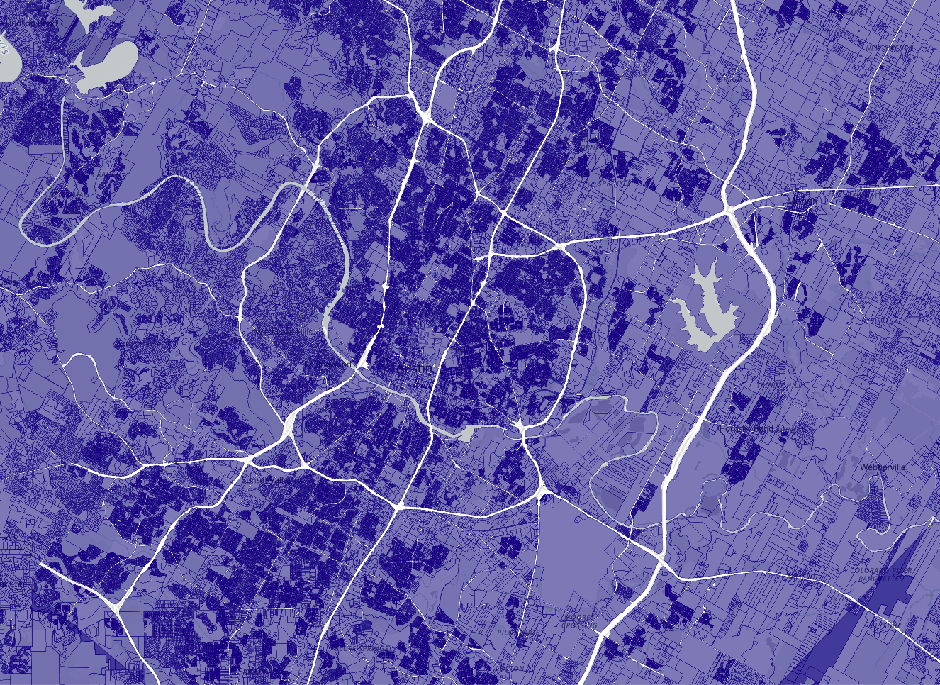
You can pick whatever port you want, but make sure to use the --cors flag to allow for cross-origin requests. We can now view our tiles on a simple map:
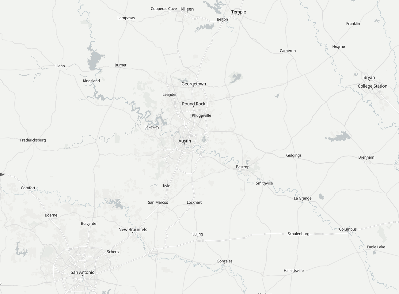
Parcels render fast and crisp due to quite a bit of internal optimization freestiler does under the hood to make it possible. However, we haven’t yet solved the last problem fully - zooming out. Our tiles start at zoom 10, so when you zoom out, you’ll see a blank map:
We’ll want to fill that space, but fortunately R and mapgl make that straightforward.
Mapping ownership in Texas by parcel
Let’s finish building out the map into something that visualizes ownership in Texas without gaps. We can pull in county geometries with the R tigris package - but since we have county information in the parcel data, let’s use our DuckDB database to calculate some interesting stats, and merge that in to the counties so we can show information when the map is zoomed out.
In the code block below, we’ll parse the owners in the parcel data, then roll up that information to the county level and pull that information into R.
We notice the counties with the largest shares of out-of-state ownership are typically smaller counties in West Texas; the exception is Travis County, where nearly 1 in 5 parcels are externally owned.
We’ll now grab county geometry from tigris and merge in our tabulated data.
library(tigris)tx_counties <-counties("TX", cb =TRUE) |>mutate(county_key =toupper(NAME)) |>left_join(county_stats, by =c("county_key"="COUNTY"))
With our county data in hand, we’ll build out the map with the mapgl package. mapgl allows you to stack and compose layers using R; it may take a few lines of code to get what you want, but mapgl exposes quite a bit of the Mapbox / MapLibre APIs. Here’s our mapping code, with some notes to follow:
I’ve written extensively about mapgl elsewhere (including on this blog), but a few features of note here.
We interpolate the county fill opacity on zoom intentionally between zoom levels 10 and 11; this creates a “fade away” effect where the counties fade away to parcels as the user zooms in. We’ll do this both for county fill and county borders (as line widths for fill layers aren’t configurable).
There are a lot of different ways to configure popups in mapgl, but one relatively new feature I’ve added is the ability to pass columns directly to popups with {column} syntax inside the popup string.
The parcel popup is set up a different way, using an overhaul to the popup engine I’ve introduced that allows for conditional popups. This is important for building highly customized popups that will differ based on the data in a given location.
I just added a new feature to mapgl that allows you to show and hide different legends on zoom with min_zoom and max_zoom arguments. So you’ll need to make sure you have the latest version of mapgl (either from GitHub or R-Universe) to use this.
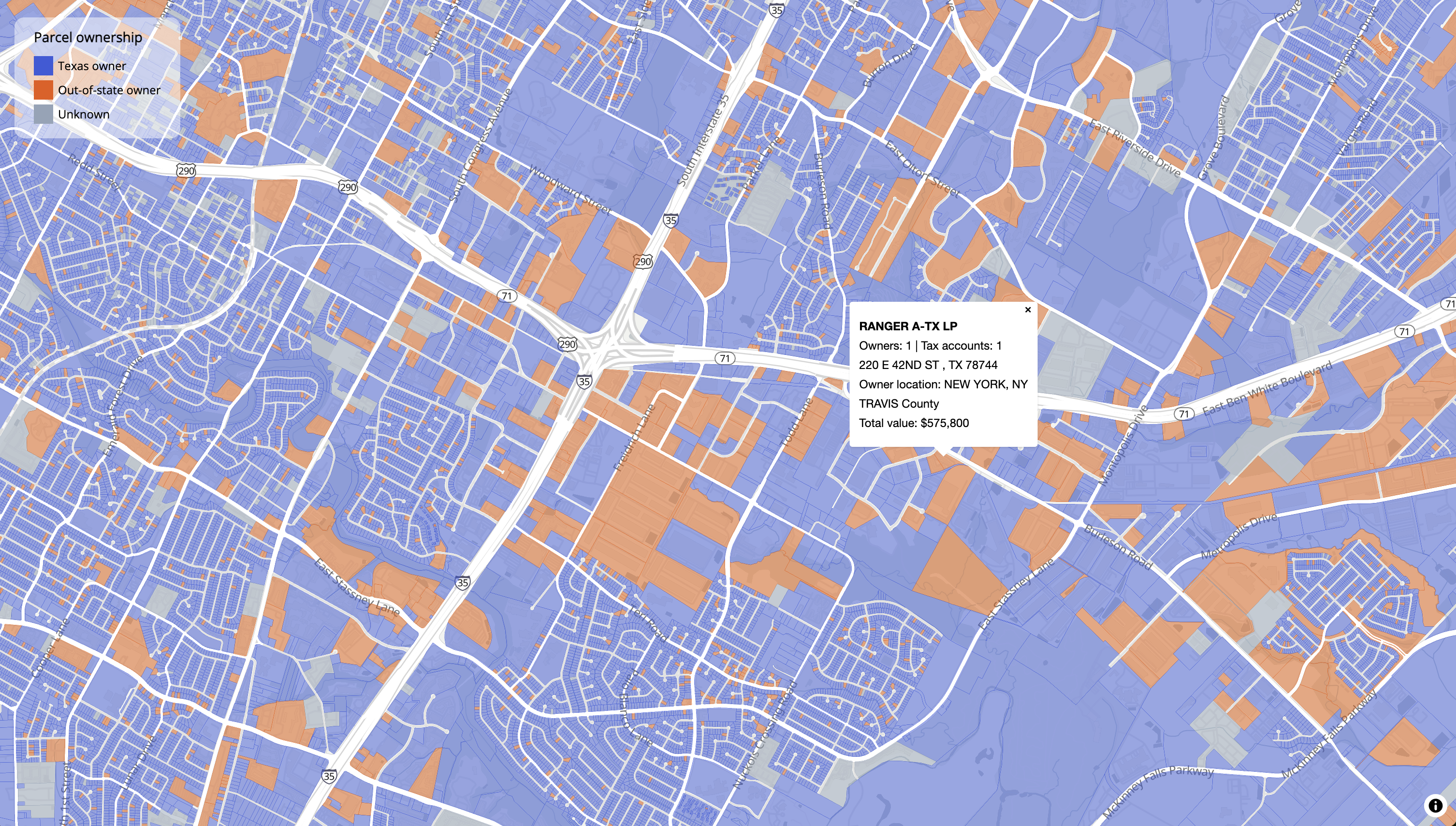
We have a map! And there’s a lot to explore. In Travis County, for example, you can find a lot of areas that have out-of-state owners, particularly around commercial corridors and on investor-owned land.
Around the state, you’ll still see some quirks of parcel data show up. Even though we consolidated duplicate geometries, you’ll still see areas with overlapping geometries. Data missingness is also an issue; for example, no parcels in Travis County carry the city name for their addresses.
The map is great - but it’s just running locally on my machine. You can’t save this out - it’s a mapping equivalent of the joke “take a look at my project, it’s at http://localhost:8002”. So we’ll need to find somewhere to host the PMTiles so we can actually share the visualization.
PMTiles is designed to work on any S3-compatible cloud storage platform that supports HTTP Range Requests. Proper support for Cross-Origin Resource Sharing is required if your map frontend is hosted on a different domain than your storage platform.
That may not mean a lot to you if you’re used to visualizing data locally on your computer. Basically, we can host our data on any number of popular cloud storage platforms (Google Cloud, Amazon S3, Microsoft Azure) so long as we configure it correctly for that specific provider. The easiest way to host PMTiles in my opinion is on GitHub Pages, which does support range requests; however, our PMTiles file is 4.7 GB in size and too large for that option. So we’ll want to upload to a cloud storage bucket.
My provider of choice is Cloudflare R2. It’s quite affordable and has zero egress fees, which means you don’t have to pay for data transfer out to the internet. Plus, if you connect a custom domain to your bucket (which you can buy through Cloudflare easily), you can use a Worker to benefit from Cloudflare’s edge caching (making it quite fast to load once set up). I’ll just show the simplest setup here.
To get started, you will need to sign up for a Cloudflare account, if you don’t have one already. You can use OAuth with Google, Apple, or GitHub, so it’s pretty painless. In the left-hand menu once you’re in, navigate to Storage & databases > R2 Object Storage. You will need to put in a credit card at this stage, but you get 10GB/month hosting for free, which means that our PMTiles will sit comfortably within the free tier.
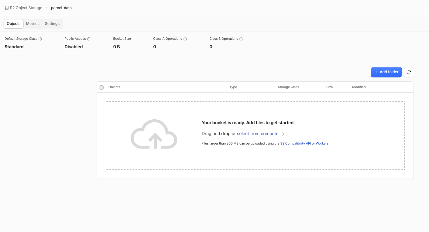
Once you’re in, look for the blue button that says Create bucket to create your first bucket. I’m naming my bucket parcel-data, but you can name yours whatever you want. Keep the other options as they are, then choose Create bucket. You’ll be taken to your bucket’s screen.
Note that you can drag-and-drop files smaller than 300MB into your bucket. For more contained PMTiles files, this is a nice option. However, our data is too big to drag-and-drop, so we’ll need to use the S3 Compatibility API. Fortunately, another one of my R packages, pmtiles, makes this straightforward.
The pmtiles package wraps the pmtiles CLI, which includes a variety of utilities for working with PMTiles files. One very useful utility is pmtiles upload which helps you upload your PMTiles files to cloud storage. In the R package, the wrapper function is pm_upload().
You’ll first need to grab a couple keys to access your bucket. Head back to the main R2 Object Storage page in Cloudflare, and look at the lower-right of the screen; you’ll see a button that says “Manage API Tokens.” Click there. Create a User API token. Give it a name, set the Permissions to “Object Read and Write,” and scope it to your specific bucket. Keep the other options as they are, then scroll down and create the token.
Copy and securely store your Access Key ID and Secret Access Key; you won’t be able to see these values again. I’d recommend putting them in your .Renviron file, which you can edit with usethis::edit_r_environ(). I’ll store mine as two lines in .Renviron: CLOUDFLARE_PARCELS_KEY and CLOUDFLARE_PARCELS_SECRET.
With these credentials in hand, we can use pm_upload() to move our data to our bucket. You’ll need one more value: your Cloudflare account ID, which is in the same Account Details panel on the R2 Object Storage page where you found the Manage API Tokens button.
The r2_bucket() helper in the pmtiles package takes it from there. R2’s S3-compatible API has some fiddly requirements - a specific URL format, a required region=auto parameter - and the helper assembles all of this correctly from just your bucket name and account ID. Your credentials are passed along to the upload process only, so they never get written into your R session’s environment variables. (There are companion helpers for other providers, too: s3_bucket(), gcs_bucket(), azure_bucket(), and s3_compatible_bucket().) Let’s upload the tiles to our bucket:
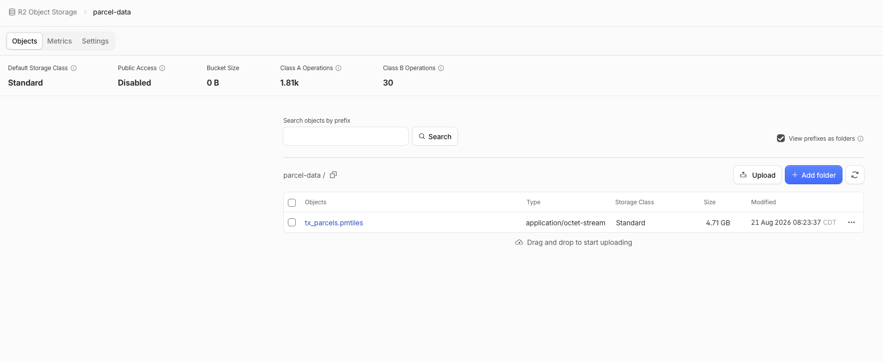
If your tiles have uploaded successfully you’ll get a success message in R. Head back to Cloudflare R2 in your web browser and you should see them there.
Now, click the Settings tab. As I mentioned earlier, if you want to deploy your data “in production” - so for a work project, or for a wide audience - you’ll want to connect a custom domain. I have a couple domains through Cloudflare that I use, and tile performance is just as fast as when I serve it on my local computer (example: https://walker-data.com/freestiler/lodes). I’ll show you here the quickest way (but not the highest-performance way) to share your tiles. Enable the Public Development URL - you’ll get a warning that this will be lower-performance than using a custom domain. Next, set the CORS policy, so your tiles can be viewed in a web map not hosted at the same domain. The CORS policy you want is this (with one caveat):
Using this block will allow any origin to access your tiles. If you’re building your maps into arbitrary projects (local work in R / Positron, various Shiny apps, etc.) this is probably what you want. However, if you do plan to share your work in a public map (and don’t want to set up a custom domain) then you might consider locking it to your site’s origin (e.g. https://walker-data.com for me).
Your PMTiles will now be accessible at {YOUR_PUBLIC_DEVELOPMENT_URL}/tx_parcels.pmtiles}, and can be used in add_pmtiles_source().
Sharing your map
With the Cloudflare setup ready to go, you’ll now be able to share your map. Use the mapping code I shared above, but swap in your deployed PMTiles URL in place of the localhost one. You should be able to see the hosted tiles in R. To share your map with others, here’s what I recommend doing:
Assign your map to a variable (e.g. m1) then write it out to disk as an HTML file with htmlwidgets::saveWidget(). If you want a single-file map use selfcontained = TRUE; I’ll recommend selfcontained = FALSE to keep your HTML smaller (just remember to move the directory together, not just the file).
m1 <-maplibre(style =openfreemap_style("positron"),center =c(-97.74, 30.27),zoom =11) |>add_pmtiles_source(id ="parcel-tiles",url ="YOUR_R2_PMTILES_URL" ) |># the rest of the mapping code follows herehtmlwidgets::saveWidget(m1, "/path/to/your/directory/index.html", selfcontained =FALSE)
Publish your map and mapping assets to your web server of choice. I like to use GitHub Pages; I host most of my websites there because it’s easy to version control my web content with git.
My live map is now available at https://walker-data.com/maps/texas-parcel-owners:
We’ve now gone end to end: downloading a 7GB geodatabase from TxGIO and visualizing those millions of parcels on a map. This tech stack (R, DuckDB, freestiler, pmtiles, and mapgl) is the same one I use in most of my projects.
One of the most important take-aways for me is not the impressive end-product but rather the series of decisions you need to make to get there. We had to figure out inconsistencies and missingness in our dataset, we had to come up with a solution for the stacked parcel problem, and we had to decide which data we were comfortable with collapsing / consolidating. These are all human decision points that are highly relevant to actual applications of this workflow, e.g. in investment, land acquisition, or right-of-way analyses. You can offload that stuff to your agent I suppose, but people who inject human expertise there are going to stand out.
Everything here transfers to your own projects, too. Florida and New York publish statewide parcel files that work with this exact pipeline, and the same pattern applies to any other massive spatial dataset you need to get on a map. Swap in your data source, make your own cleaning decisions, and keep the plumbing.
Finally - if your team works with parcel, ownership, or land data and wants to build workflows like this, this is exactly what I do. Reach out to kyle@walker-data.com to discuss your idea. And if you make something with this stack, let me know what you create!