library(tigris)
library(dplyr)
library(pmtiles)
library(mapgl)
library(sf)
options(tigris_use_cache = TRUE)

tx_blocks <- blocks(state = "TX", year = 2024)

nrow(tx_blocks)Mapping 650,000+ Texas Census blocks with PMTiles
r
gis
census
mapping
I’ve been working on the mapgl R package for the past year which brings high-performance WebGL mapping to R users. While Mapbox and MapLibre are impressive libraries, the traditional way mapgl visualizes vector datasets - as GeoJSON sources - runs into bottlenecks with very large datasets. If you are dealing with millions of points, or hundreds of thousands of polygons, your map may render slowly (or not render at all).
In these instances, I’ve had a lot of success with PMTiles. PMTiles is a single-file archive format for tiled map data that can transform your work with large geospatial data visualization. I’m using PMTiles to visualize millions of features in production mapping applications quickly and efficiently.
This is the first of a three-post series that steps you through the process of working with PMTiles in your mapping applications. In this post, I’ll introduce you to my brand-new pmtiles R package, which provides an R wrapper for the PMTiles command-line tool along with some other utilities for creating and viewing PMTiles. I’ll show you how to map all 655,000+ Census blocks in Texas - complete with 3D extrusion, hover effects, and tooltips - all locally on your computer.
The second and third posts in this series will focus on moving PMTiles workflows to production. In the second post, I’ll walk you through how to deploy your PMTiles to Cloudflare R2 so you can share your maps with the world. In the third post, I’ll show you how to integrate your tiles into a Shiny web mapping application and deploy your app for production use.
Getting Census block data with tigris
Let’s start by grabbing Census block boundaries for Texas using the tigris package. Census blocks are the smallest geographic unit published by the Census Bureau - and Texas has more of them than any other state.
We’ve got 668,757 blocks. That’s a lot of polygons to visualize on a map!
Let’s clean up the data a bit. We’ll select the columns we care about, filter out water-only blocks, and calculate some derived measures like population density.
tx_blocks_cleaned <- tx_blocks |>
  select(
    geoid = GEOID20,
    area_land = ALAND20,
    area_water = AWATER20,
    housing = HOUSING20,
    population = POP20
  ) |>
  filter(area_land > 0) |>
  mutate(
    pop_density = population / (area_land / 2589988),
    housing_density = housing / (area_land / 2589988)
  )

nrow(tx_blocks_cleaned)
After removing water-only blocks, we’re down to 655,142 blocks. Still a massive dataset to visualize!
Creating PMTiles with pm_create()
The pmtiles package includes pm_create(), which wraps the tippecanoe tool for creating high-quality tiled map archives. You’ll need to install tippecanoe separately (on macOS: brew install tippecanoe; see the package README for other platforms).
The simplest way to create a tileset is to specify an input dataset and output PMTiles file, then let tippecanoe choose the rest of the arguments.
pm_create(tx_blocks_cleaned, "tx_blocks_default.pmtiles")pm_create() works directly with sf objects and handles all the complexity of tile generation behind the scenes. tippecanoe needs to process all of the Census blocks into tiles, so this process may take a few minutes to complete. When your tiles are ready, you can preview them with pm_view():
pm_view("tx_blocks_default.pmtiles")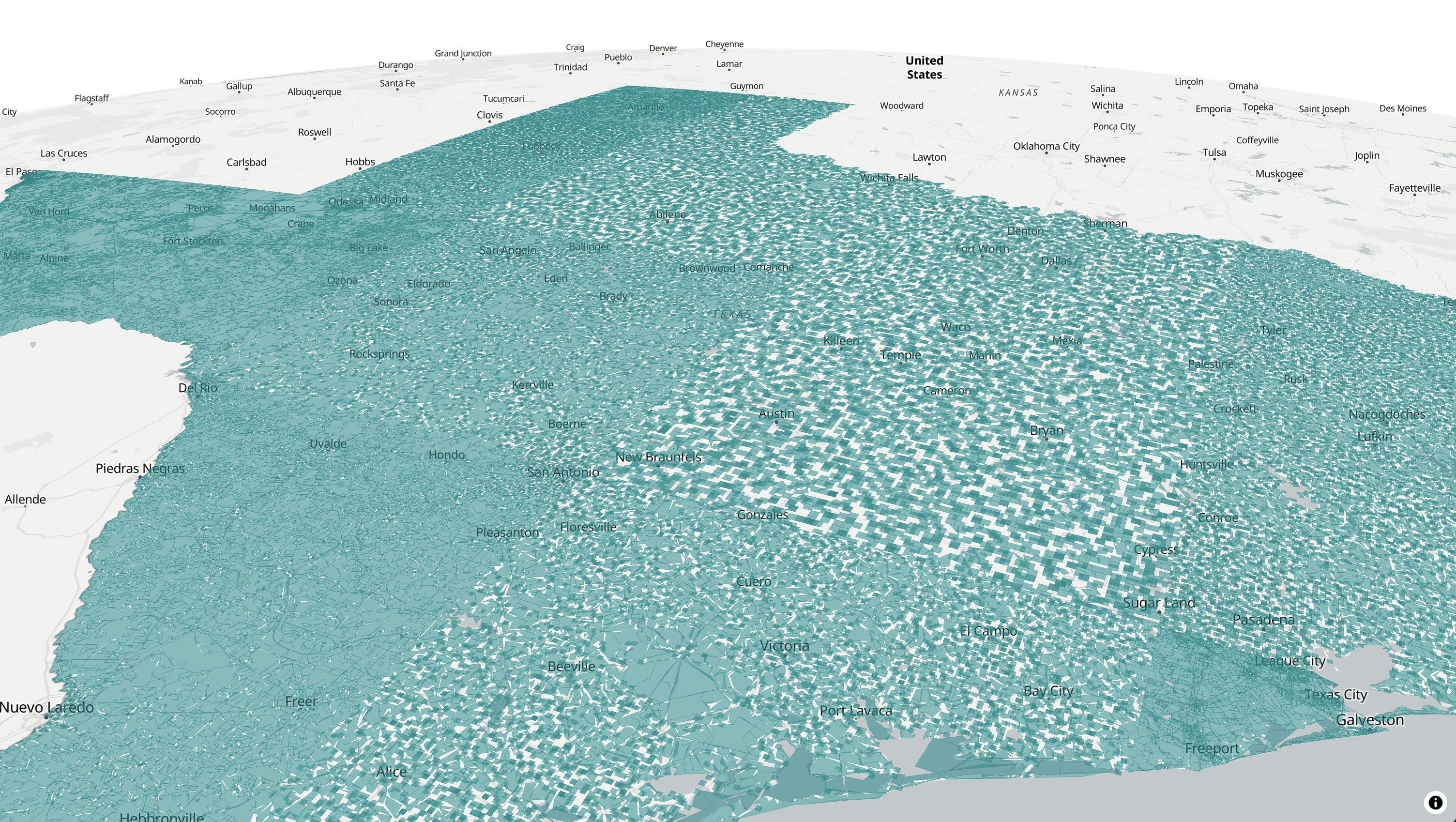
We notice that the data can be explored very quickly, but the blocks are very choppy when zoomed out. This is because the default options for tippecanoe are optimizing the tileset for display and performance; you’ll notice that all blocks become fully formed when you zoom in.
In many cases, this configuration may be fine. In another post, I discussed the value of zoom-dependent layering to govern the data that is displayed by zoom level. In your map, you might display larger geographies (e.g. counties, Census tracts) at small zooms, then give way to blocks when zoomed in.
tippecanoe can be configured to avoid dropping features, however. The pm_create() function is designed to expose the multitude of tippecanoe’s options to R users. The recipe below will create a denser tileset that preserves all features; we’ll start the tileset at zoom level 8 and build tiles through zoom level 14.
Here’s how we do it:
pm_create(
  tx_blocks_cleaned,
  "tx_blocks.pmtiles",
  layer_name = "blocks",
  min_zoom = 8,
  max_zoom = 14,
  no_tiny_polygon_reduction = TRUE,
  no_tile_size_limit = TRUE,
  no_feature_limit = TRUE,
  simplification = 2,
  detect_shared_borders = TRUE,
  generate_ids = TRUE
)
Let’s walk through what these options do:
min_zoom = 8means blocks will start appearing when zoomed in to a metro-area level viewmax_zoom = 14gives us good detail without generating tiles we’ll never useno_tiny_polygon_reduction = TRUEprevents tippecanoe from dropping small polygonsno_tile_size_limit = TRUEallows larger tile sizes to accommodate all featuresno_feature_limit = TRUEensures all blocks are included at every zoom levelsimplification = 2applies minimal geometry simplification at lower zoom levelsdetect_shared_borders = TRUEensures adjacent blocks share borders cleanlygenerate_ids = TRUEis needed for interactivity (hover effects, tooltips)
These options create a larger PMTiles file, but eliminate the holes that appear when features are dropped. The result is a single tx_blocks.pmtiles file with complete coverage, ready to visualize.
Inspecting features with pm_view()
pm_view() includes an argument inspect_features that will show the properties of any hovered-over feature in a tooltip. Let’s try this out on our dense tileset and customize the color:
pm_stop_server()

pm_view("tx_blocks.pmtiles", inspect_features = TRUE, fill_color = "red")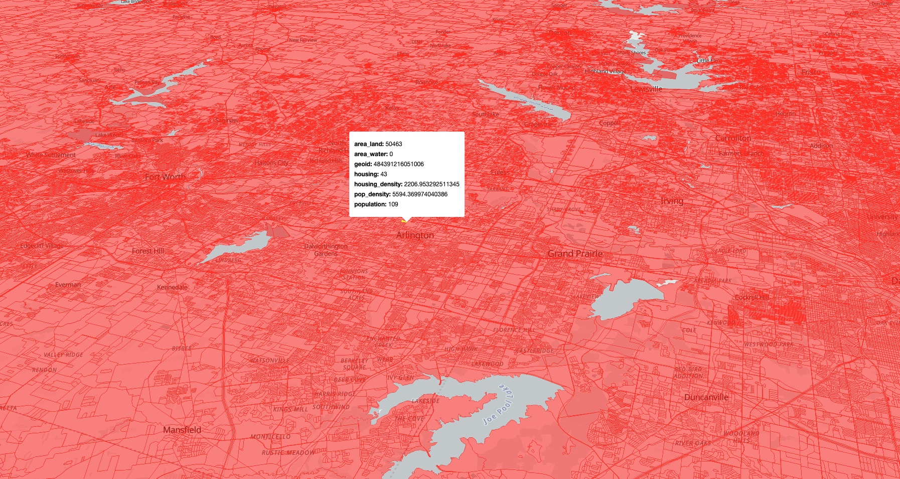
This gives you an interactive map with hover tooltips showing all the attributes for each block. Performance will be slightly slower than with our first dataset, but you’ll notice that there are no longer holes - and your data still can be browsed very quickly.
pm_view() by default spins up a local server using httpuv to serve the tileset locally, then maps it with MapLibre. Our tileset is small enough to work well with this approach, but I’ve found that httpuv can struggle with tilesets of size 1GB and up.
In these cases, I like to use Node’s http-server instead (serving here on port 3131), then pass the URL to pm_view():
npm install -g http-server

http-server -p 3131 --cors
Then in R:
pm_view("http://localhost:3131/tx_blocks.pmtiles", inspect_features = TRUE)Custom visualization with mapgl
While pm_view() is great for quick previews, the real power comes from building custom visualizations with the mapgl package. Let’s create a 3D visualization that extrudes blocks based on population density and colors them by population.
First, we’ll start a local server for our PMTiles file:
pm_serve("tx_blocks.pmtiles", port = 8888)Then we can build our custom map. We’ll pass the URL to mapgl’s add_pmtiles_source(), then style it downstream as a fill extrusion layer.
maplibre(
  style = openfreemap_style("dark"),
  center = c(-96.8, 32.7),
  zoom = 10,
  pitch = 45,
  hash = TRUE
) |>
  add_pmtiles_source(
    id = "blocks",
    url = "http://localhost:8888/tx_blocks.pmtiles"
  ) |>
  add_fill_extrusion_layer(
    id = "blocks-3d",
    source = "blocks",
    source_layer = "blocks",
    fill_extrusion_height = interpolate(
      column = "pop_density",
      values = c(0, 50000),
      stops = c(0, 5000)
    ),
    fill_extrusion_color = interpolate(
      column = "population",
      values = c(0, 50, 100, 250, 1000),
      stops = RColorBrewer::brewer.pal(5, "PuRd")
    ),
    hover_options = list(
      fill_extrusion_color = "cyan"
    ),
    tooltip = concat(
      "Block: ",
      get_column("geoid"),
      "<br>",
      "Population: ",
      get_column("population"),
      "<br>",
      "Housing units: ",
      get_column("housing")
    )
  )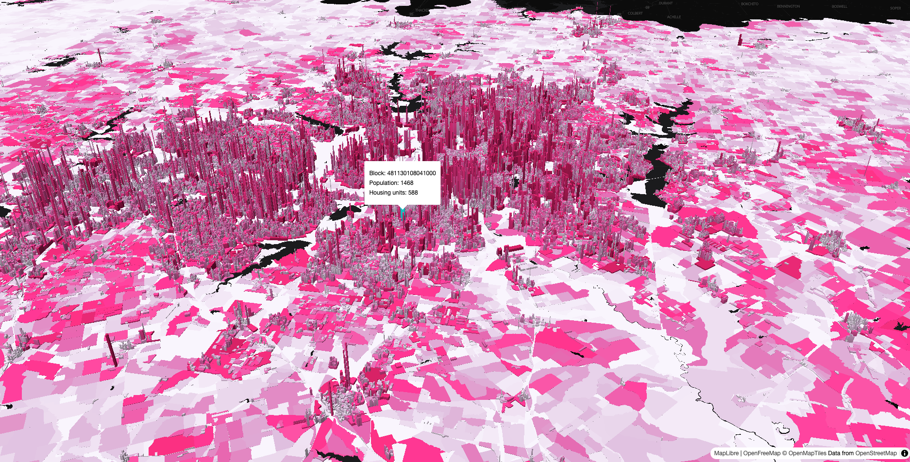
The 3D extrusion gives us an immediate sense of where population is concentrated in the Dallas-Fort Worth area. The extrusion height is based on population density, and the color represents total population. Hover over any block to see its specific attributes, then browse around Texas! The hash = TRUE parameter adds the map state to the URL, so you can share specific views with others.
Next steps
We’ve mapped 655,000 Census blocks without a database or dedicated tile server - just R, PMTiles, and local file serving. The workflow from raw data to interactive 3D map takes minutes, and the resulting PMTiles file is a portable, single-file archive that integrates really well with web mapping tools like MapLibre.
In Part II of this series, I’ll show you how to deploy PMTiles to the cloud with Cloudflare R2, including both simple public deployments with pm_upload() and more complex setups using Cloudflare Workers for secure data that you don’t want fully downloadable. In Part III, we’ll then integrate our PMTiles visualization into a dynamic Shiny web mapping application, and discuss options for deploying your PMTiles app for production use.
If you want to try this workflow yourself, check out the pmtiles package and let me know what you create!