Analyzing Data from the 2023 American Community Survey in R
2025-02-05
About me
Professor of Geography at TCU
Spatial data science researcher and consultant
Package developer: tidycensus, tigris, mapgl, mapboxapi, crsuggest, idbr (R), pygris (Python)
Book: Analyzing US Census Data: Methods, Maps and Models in R
SSDAN webinar series
Today: Analyzing Data from the 2023 American Community Survey in R
Wednesday, February 12th: Working with Decennial Census Data in R
Wednesday, February 26th: Mapping and Spatial Analysis with US Census Data in R
Today’s agenda
Hour 1: The American Community Survey, R, and tidycensus
Hour 2: ACS data workflows
Hour 3: An introduction to ACS microdata
The American Community Survey, R, and tidycensus
What is the ACS?
Annual survey of 3.5 million US households
Covers topics not available in decennial US Census data (e.g. income, education, language, housing characteristics)
Available as 1-year estimates (for geographies of population 65,000 and greater) and 5-year estimates (for geographies down to the block group)
Data delivered as estimates characterized by margins of error
How to get ACS data
data.census.gov is the main, revamped interactive data portal for browsing and downloading Census datasets, including the ACS
The US Census Application Programming Interface (API) allows developers to access Census data resources programmatically
tidycensus
R interface to the Decennial Census, American Community Survey, Population Estimates Program, and Public Use Microdata Series APIs
First released in 2017; nearly 600,000 downloads from the Posit CRAN mirror
![]()
tidycensus: key features
Wrangles Census data internally to return tidyverse-ready format (or traditional wide format if requested);
Automatically downloads and merges Census geometries to data for mapping;
Includes tools for handling margins of error in the ACS and working with survey weights in the ACS PUMS;
States and counties can be requested by name (no more looking up FIPS codes!)
R and RStudio
R: programming language and software environment for data analysis (and wherever else your imagination can take you!)
RStudio: integrated development environment (IDE) for R developed by Posit
Posit Cloud: run RStudio with today’s workshop pre-configured at https://posit.cloud/content/9689451
Getting started with tidycensus
To get started, install the packages you’ll need for today’s workshop
If you are using the Posit Cloud environment, these packages are already installed for you
- Optional, to run advanced examples:
Optional: your Census API key
tidycensus (and the Census API) can be used without an API key, but you will be limited to 500 queries per day
Power users: visit https://api.census.gov/data/key_signup.html to request a key, then activate the key from the link in your email.
Once activated, use the
census_api_key()function to set your key as an environment variableAs of February 2025, the API key service appears to be unavailable
Getting started with ACS data in tidycensus
Using the get_acs() function
The
get_acs()function is your portal to access ACS data using tidycensusThe two required arguments are
geographyandvariables. As of v1.7.1, the function defaults to the 2019-2023 5-year ACS
- ACS data are returned with five columns:
GEOID,NAME,variable,estimate, andmoe
# A tibble: 3,222 × 5
GEOID NAME variable estimate moe
<chr> <chr> <chr> <dbl> <dbl>
1 01001 Autauga County, Alabama B25077_001 197900 8280
2 01003 Baldwin County, Alabama B25077_001 287000 6910
3 01005 Barbour County, Alabama B25077_001 109900 11374
4 01007 Bibb County, Alabama B25077_001 132600 18638
5 01009 Blount County, Alabama B25077_001 169700 5354
6 01011 Bullock County, Alabama B25077_001 79400 15850
7 01013 Butler County, Alabama B25077_001 99700 8484
8 01015 Calhoun County, Alabama B25077_001 149500 6196
9 01017 Chambers County, Alabama B25077_001 129700 12036
10 01019 Cherokee County, Alabama B25077_001 165900 9786
# ℹ 3,212 more rows1-year ACS data
1-year ACS data are more current, but are only available for geographies of population 65,000 and greater
Access 1-year ACS data with the argument
survey = "acs1"; defaults to"acs5"
# A tibble: 649 × 5
GEOID NAME variable estimate moe
<chr> <chr> <chr> <dbl> <dbl>
1 0103076 Auburn city, Alabama B25077_001 365500 39357
2 0107000 Birmingham city, Alabama B25077_001 157200 14921
3 0121184 Dothan city, Alabama B25077_001 190000 10687
4 0135896 Hoover city, Alabama B25077_001 415300 20389
5 0137000 Huntsville city, Alabama B25077_001 309900 15846
6 0150000 Mobile city, Alabama B25077_001 189000 20112
7 0151000 Montgomery city, Alabama B25077_001 158500 8737
8 0177256 Tuscaloosa city, Alabama B25077_001 252200 26811
9 0203000 Anchorage municipality, Alaska B25077_001 385900 11025
10 0404720 Avondale city, Arizona B25077_001 404900 17356
# ℹ 639 more rowsRequesting tables of variables
- The
tableparameter can be used to obtain all related variables in a “table” at once
# A tibble: 54,774 × 5
GEOID NAME variable estimate moe
<chr> <chr> <chr> <dbl> <dbl>
1 01001 Autauga County, Alabama B19001_001 22523 431
2 01001 Autauga County, Alabama B19001_002 831 221
3 01001 Autauga County, Alabama B19001_003 676 211
4 01001 Autauga County, Alabama B19001_004 801 312
5 01001 Autauga County, Alabama B19001_005 984 281
6 01001 Autauga County, Alabama B19001_006 983 322
7 01001 Autauga County, Alabama B19001_007 1057 255
8 01001 Autauga County, Alabama B19001_008 768 241
9 01001 Autauga County, Alabama B19001_009 961 266
10 01001 Autauga County, Alabama B19001_010 837 248
# ℹ 54,764 more rowsUnderstanding geography and variables in tidycensus
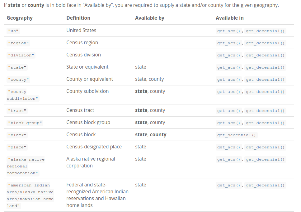
US Census Geography
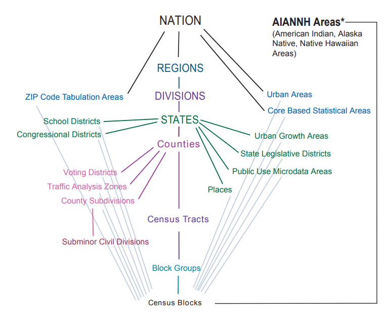
Geography in tidycensus
- Information on available geographies, and how to specify them, can be found in the tidycensus documentation
Querying by state
For geographies available below the state level, the
stateparameter allows you to query data for a specific stateFor smaller geographies (Census tracts, block groups), a
countycan also be requestedtidycensus translates state names and postal abbreviations internally, so you don’t need to remember the FIPS codes!
Example: data on median home value in San Diego County, California by Census tract
# A tibble: 737 × 5
GEOID NAME variable estimate moe
<chr> <chr> <chr> <dbl> <dbl>
1 06073000100 Census Tract 1; San Diego County; Calif… B25077_… 1825500 159981
2 06073000201 Census Tract 2.01; San Diego County; Ca… B25077_… 1445900 203254
3 06073000202 Census Tract 2.02; San Diego County; Ca… B25077_… 966200 175650
4 06073000301 Census Tract 3.01; San Diego County; Ca… B25077_… 895600 152793
5 06073000302 Census Tract 3.02; San Diego County; Ca… B25077_… 820800 132232
6 06073000400 Census Tract 4; San Diego County; Calif… B25077_… 802500 108414
7 06073000500 Census Tract 5; San Diego County; Calif… B25077_… 1031800 96156
8 06073000600 Census Tract 6; San Diego County; Calif… B25077_… 723300 78902
9 06073000700 Census Tract 7; San Diego County; Calif… B25077_… 833900 107773
10 06073000800 Census Tract 8; San Diego County; Calif… B25077_… 795900 246242
# ℹ 727 more rowsSearching for variables
To search for variables, use the
load_variables()function along with a year and datasetThe
View()function in RStudio allows for interactive browsing and filtering
Available ACS datasets in tidycensus
Detailed Tables
Data Profile (add
"/profile"for variable lookup)Subject Tables (add
"/subject")Comparison Profile (add
"/cprofile")Supplemental Estimates (use
"acsse")Migration Flows (access with
get_flows())
“Tidy” or long-form data
# A tibble: 2,548 × 5
GEOID NAME variable estimate moe
<chr> <chr> <chr> <dbl> <dbl>
1 01 Alabama B01001_001 5108468 NA
2 01 Alabama B01001_002 2471801 5359
3 01 Alabama B01001_003 143309 3322
4 01 Alabama B01001_004 154161 6072
5 01 Alabama B01001_005 169656 6167
6 01 Alabama B01001_006 104280 3039
7 01 Alabama B01001_007 73719 3352
8 01 Alabama B01001_008 33655 3913
9 01 Alabama B01001_009 32913 3242
10 01 Alabama B01001_010 100629 5077
# ℹ 2,538 more rows“Wide” data
# A tibble: 52 × 100
GEOID NAME B01001_001E B01001_001M B01001_002E B01001_002M B01001_003E
<chr> <chr> <dbl> <dbl> <dbl> <dbl> <dbl>
1 01 Alabama 5108468 NA 2471801 5359 143309
2 02 Alaska 733406 NA 385855 2547 24360
3 04 Arizona 7431344 NA 3708672 2905 198924
4 05 Arkansas 3067732 NA 1512201 4594 89183
5 06 California 38965193 NA 19450698 5477 1067828
6 08 Colorado 5877610 NA 2980108 4746 159079
7 09 Connecticut 3617176 NA 1775718 2410 92614
8 10 Delaware 1031890 NA 498994 1839 26971
9 11 District o… 678972 NA 321590 265 19516
10 12 Florida 22610726 NA 11116575 6588 577538
# ℹ 42 more rows
# ℹ 93 more variables: B01001_003M <dbl>, B01001_004E <dbl>, B01001_004M <dbl>,
# B01001_005E <dbl>, B01001_005M <dbl>, B01001_006E <dbl>, B01001_006M <dbl>,
# B01001_007E <dbl>, B01001_007M <dbl>, B01001_008E <dbl>, B01001_008M <dbl>,
# B01001_009E <dbl>, B01001_009M <dbl>, B01001_010E <dbl>, B01001_010M <dbl>,
# B01001_011E <dbl>, B01001_011M <dbl>, B01001_012E <dbl>, B01001_012M <dbl>,
# B01001_013E <dbl>, B01001_013M <dbl>, B01001_014E <dbl>, …Using named vectors of variables
Census variables can be hard to remember; using a named vector to request variables will replace the Census IDs with a custom input
In long form, these custom inputs will populate the
variablecolumn; in wide form, they will replace the column names
# A tibble: 174 × 5
GEOID NAME variable estimate moe
<chr> <chr> <chr> <dbl> <dbl>
1 06001 Alameda County, California percent_high_school 15.9 0.3
2 06001 Alameda County, California percent_bachelors 28.7 0.3
3 06001 Alameda County, California percent_graduate 22.8 0.3
4 06003 Alpine County, California percent_high_school 18.5 6.1
5 06003 Alpine County, California percent_bachelors 22.4 7.3
6 06003 Alpine County, California percent_graduate 19.7 9.3
7 06005 Amador County, California percent_high_school 26.5 1.6
8 06005 Amador County, California percent_bachelors 15.5 1.5
9 06005 Amador County, California percent_graduate 7 1.1
10 06007 Butte County, California percent_high_school 22.3 0.8
# ℹ 164 more rowsPart 1 exercises
Use the
load_variables()function to find a variable that interests you that we haven’t used yet.Use
get_acs()to fetch data on that variable from the ACS for counties, similar to how we did for median household income.
Part 2: ACS data workflows
Understanding limitations of the 1-year ACS
- The 1-year American Community Survey is only available for geographies with population 65,000 and greater. This means:
- Only 854 of 3,222 counties are available
- Only 649 of 32,325 cities / Census-designated places are available
- No data for Census tracts, block groups, ZCTAs, or any other geographies that typically have populations below 65,000
Data sparsity and margins of error
- You may encounter data issues in the 1-year ACS data that are less pronounced in the 5-year ACS. For example:
Values available in the 5-year ACS may not be available in the corresponding 1-year ACS tables
If available, they will likely have larger margins of error
Your job as an analyst: balance need for certainty vs. need for recency in estimates
Example: Punjabi speakers by state (1-year ACS)
# A tibble: 52 × 5
GEOID NAME variable estimate moe
<chr> <chr> <chr> <dbl> <dbl>
1 01 Alabama B16001_054 1149 947
2 02 Alaska B16001_054 NA NA
3 04 Arizona B16001_054 2180 1477
4 05 Arkansas B16001_054 0 208
5 06 California B16001_054 171384 13741
6 08 Colorado B16001_054 1997 1973
7 09 Connecticut B16001_054 2062 1095
8 10 Delaware B16001_054 1643 1814
9 11 District of Columbia B16001_054 67 74
10 12 Florida B16001_054 5148 2555
# ℹ 42 more rowsPunjabi speakers by state (5-year ACS)
# A tibble: 52 × 5
GEOID NAME variable estimate moe
<chr> <chr> <chr> <dbl> <dbl>
1 01 Alabama B16001_054 704 321
2 02 Alaska B16001_054 0 24
3 04 Arizona B16001_054 2824 594
4 05 Arkansas B16001_054 519 257
5 06 California B16001_054 151139 6187
6 08 Colorado B16001_054 1406 505
7 09 Connecticut B16001_054 1945 529
8 10 Delaware B16001_054 236 176
9 11 District of Columbia B16001_054 39 34
10 12 Florida B16001_054 2959 764
# ℹ 42 more rowsVisualizing ACS data
Visualizing ACS estimates
As opposed to decennial US Census data, ACS estimates include information on uncertainty, represented by the margin of error in the
moecolumnThis means that in some cases, visualization of estimates without reference to the margin of error can be misleading
Walkthrough: building a margin of error visualization with ggplot2
Visualizing ACS estimates
- Let’s get some data on median household income by county in Utah
A basic plot
- To visualize a dataset with ggplot2, we define an aesthetic and a geom

Problems with our basic plot
The data are not sorted by value, making comparisons difficult
The axis and tick labels are not intuitive
The Y-axis labels contain repetitive information (” County, Utah”)
We’ve made no attempt to customize the styling
Sorting by value
- We use
reorder()to sort counties by the value of their ACS estimates, improving legibility

Cleaning up tick labels
- Using a combination of functions in the scales package and custom-defined functions, tick labels can be formatted any way you want

Improving formatting and theming
- Use
labs()to label the plot and its axes, and change the theme to one of several built-in options

Problem: comparing ACS estimates
- The chart suggests that Juab County has lower income than Salt Lake County but its margin of error is quite large
- How to visualize uncertainty in an intuitive way?
Visualizing margins of error
utah_plot_errorbar <- ggplot(utah_income, aes(x = estimate,
y = reorder(NAME, estimate))) +
geom_errorbar(aes(xmin = estimate - moe, xmax = estimate + moe), #<<
width = 0.5, linewidth = 0.5) + #<<
geom_point(color = "darkblue", size = 2) +
scale_x_continuous(labels = label_dollar()) +
scale_y_discrete(labels = function(x) str_remove(x, " County, Utah")) +
labs(title = "Median household income, 2019-2023 ACS",
subtitle = "Counties in Utah",
caption = "Data acquired with R and tidycensus. Error bars represent margin of error around estimates.",
x = "ACS estimate",
y = "") +
theme_minimal(base_size = 12)
Exploring maps of ACS data
“Spatial” ACS data
One of the best features of tidycensus is the argument
geometry = TRUE, which gets you the correct Census geometries with no hassleget_acs()withgeometry = TRUEreturns a spatial Census dataset containing simple feature geometriesAs of February 2025, the Census geographic shapefiles used by tidycensus have been taken offline, so we’ll be taking a look at some workarounds
“Spatial” ACS data
Geometry workaround
- Corresponding geometries are available from the TigerWeb API, accessed with the {arcgislayers} package
- We get back a simple features data frame (more about this on February 26th)
Simple feature collection with 1331 features and 17 fields
Geometry type: POLYGON
Dimension: XY
Bounding box: xmin: -9825464 ymin: 5081873 xmax: -9743145 ymax: 5184116
Projected CRS: WGS 84 / Pseudo-Mercator
First 10 features:
MTFCC OID GEOID STATE COUNTY TRACT BASENAME
1 G5020 207903704492010 17031030101 17 031 030101 301.01
2 G5020 207903704492021 17031030701 17 031 030701 307.01
3 G5020 207903704492051 17031070103 17 031 070103 701.03
4 G5020 20790197959947 17031807100 17 031 807100 8071
5 G5020 20790197959946 17031807200 17 031 807200 8072
6 G5020 20790197959945 17031807300 17 031 807300 8073
7 G5020 20790197959944 17031807400 17 031 807400 8074
8 G5020 20790197959943 17031807500 17 031 807500 8075
9 G5020 20790197959941 17031807700 17 031 807700 8077
10 G5020 20790197959939 17031807900 17 031 807900 8079
NAME LSADC FUNCSTAT AREALAND AREAWATER OBJECTID CENTLAT
1 Census Tract 301.01 CT S 127283 110999 8482 +41.9912045
2 Census Tract 307.01 CT S 69878 0 8483 +41.9827453
3 Census Tract 701.03 CT S 69094 0 8484 +41.9268213
4 Census Tract 8071 CT S 1528033 0 8487 +42.0444541
5 Census Tract 8072 CT S 2489125 0 8488 +42.0371765
6 Census Tract 8073 CT S 2037391 0 8514 +42.0337542
7 Census Tract 8074 CT S 1396762 0 8515 +42.0281982
8 Census Tract 8075 CT S 988887 0 8516 +42.0279560
9 Census Tract 8077 CT S 1697095 0 8955 +42.0207253
10 Census Tract 8079 CT S 2013730 0 8956 +42.0041682
CENTLON INTPTLAT INTPTLON geometry
1 -087.6573633 +41.9910538 -087.6548790 POLYGON ((-9758304 5159824,...
2 -087.6579659 +41.9827453 -087.6579659 POLYGON ((-9758274 5158526,...
3 -087.6426050 +41.9268110 -087.6426051 POLYGON ((-9756510 5150208,...
4 -087.7210876 +42.0444535 -087.7210786 POLYGON ((-9766345 5167360,...
5 -087.7285090 +42.0371751 -087.7285103 POLYGON ((-9767978 5166271,...
6 -087.7548822 +42.0337614 -087.7549133 POLYGON ((-9769870 5166885,...
7 -087.7398421 +42.0281935 -087.7398439 POLYGON ((-9767999 5165384,...
8 -087.7281340 +42.0279578 -087.7281380 POLYGON ((-9766395 5164912,...
9 -087.7542264 +42.0207639 -087.7542195 POLYGON ((-9770177 5164408,...
10 -087.7487805 +42.0041886 -087.7487798 POLYGON ((-9769616 5161377,...Tutorial: using TIGERweb
- Link: https://tigerweb.geo.census.gov/tigerwebmain/TIGERweb_main.html
Spatial ACS data
- With the geometries in hand, we can merge the ACS data using
left_join()
library(dplyr)
cook_education_geo <- cook_geo %>%
select(GEOID) %>%
left_join(cook_education, by = "GEOID")
cook_education_geoSimple feature collection with 1331 features and 5 fields
Geometry type: POLYGON
Dimension: XY
Bounding box: xmin: -9825464 ymin: 5081873 xmax: -9743145 ymax: 5184116
Projected CRS: WGS 84 / Pseudo-Mercator
First 10 features:
GEOID NAME variable estimate
1 17031030101 Census Tract 301.01; Cook County; Illinois DP02_0068P 50.0
2 17031030701 Census Tract 307.01; Cook County; Illinois DP02_0068P 48.2
3 17031070103 Census Tract 701.03; Cook County; Illinois DP02_0068P 88.4
4 17031807100 Census Tract 8071; Cook County; Illinois DP02_0068P 73.2
5 17031807200 Census Tract 8072; Cook County; Illinois DP02_0068P 52.7
6 17031807300 Census Tract 8073; Cook County; Illinois DP02_0068P 52.5
7 17031807400 Census Tract 8074; Cook County; Illinois DP02_0068P 49.8
8 17031807500 Census Tract 8075; Cook County; Illinois DP02_0068P 48.0
9 17031807700 Census Tract 8077; Cook County; Illinois DP02_0068P 44.1
10 17031807900 Census Tract 8079; Cook County; Illinois DP02_0068P 63.3
moe geometry
1 9.5 POLYGON ((-9758304 5159824,...
2 6.1 POLYGON ((-9758274 5158526,...
3 5.3 POLYGON ((-9756510 5150208,...
4 6.5 POLYGON ((-9766345 5167360,...
5 7.0 POLYGON ((-9767978 5166271,...
6 7.1 POLYGON ((-9769870 5166885,...
7 8.1 POLYGON ((-9767999 5165384,...
8 6.7 POLYGON ((-9766395 5164912,...
9 6.8 POLYGON ((-9770177 5164408,...
10 7.8 POLYGON ((-9769616 5161377,...Exploring spatial data
Mapping, GIS, and spatial data is the subject of our February 26 workshop - so be sure to check that out!
Even before we dive deeper into spatial data, it is very useful to be able to explore your results on an interactive map
Our solution:
mapview()
Exploring spatial data
Creating a shaded map with zcol
What about mapping 1-year ACS data?
- Typically it is difficult to map 1-year ACS data below the state level as your data will have gaps due to the population restrictions
Example: “mapping” 1-year ACS data
tx_education <- get_acs(
geography = "county",
variables = "DP02_0068P",
state = "TX",
year = 2023,
survey = "acs1"
)
tx_counties <- arc_read("https://tigerweb.geo.census.gov/arcgis/rest/services/Generalized_ACS2023/State_County/MapServer/11", where = "STATE = '48'")
tx_geo <- left_join(tx_counties, tx_education, by = "GEOID")Example: “mapping” 1-year ACS data
Mapping small(er) areas with PUMAs
Consider using Public Use Microdata Areas (PUMAs) for geographically-consistent substate mapping
PUMAs are typically used for microdata geography; however, I find them quite useful to approximate real state submarkets, planning areas, etc.
tx_wfh <- get_acs(
geography = "puma",
variables = "DP03_0024P",
state = "TX",
survey = "acs1",
year = 2023
)
tx_pumas <- arc_read("https://tigerweb.geo.census.gov/arcgis/rest/services/Generalized_TAB2020/PUMA_TAD_TAZ_UGA_ZCTA/MapServer/4", where = "STATE = '48'")
tx_geo <- left_join(tx_pumas, tx_wfh, by = "GEOID")Time-series analysis with the 1-year ACS: some notes
Variables in the Data Profile and Subject Tables can change names over time
You’ll need to watch out for the Connecticut issue and changing geographies
The 2020 1-year ACS was not released (and is not in tidycensus), so your time-series can break if you are using iteration to pull data
Part 2 exercises
Swap in a variable from Part 1, "B25077_001" (median home value) for the analysis in this section, and try the following:
For a state of your choosing, how do margins of error differ among counties for median home values in the 1-year and 5-year ACS?
Can you visualize trends in median home value for a county of your choosing using
mapview()?
Part 3: Working with ACS microdata
What is “microdata?”
Microdata: individual-level survey responses made available to researchers
The ACS Public Use Microdata Series (PUMS) allows for detailed cross-tabulations not available in aggregated data
The 1-year PUMS covers about 1 percent of the US population; the 5-year PUMS covers about 5 percent (so, not the full ACS)
Data downloads available in bulk from the Census FTP server or from data.census.gov’s MDAT tool
Other resource for cleaned, time-series microdata: IPUMS
Using microdata in tidycensus
Basic usage of get_pums()
get_pums()requires specifying one or more variables and the state for which you’d like to request data.state = 'all'can get data for the entire USA, but it takes a while!The function defaults to the 5-year ACS with
survey = "acs5"; 1-year ACS data is available withsurvey = "acs1".The default year is 2023 in the latest version of tidycensus; data are available back to 2005 (1-year ACS) and 2005-2009 (5-year ACS). 2020 1-year data are not available.
Basic usage of get_pums()
# A tibble: 45,026 × 8
SERIALNO SPORDER WGTP PWGTP AGEP STATE HHT SEX
<chr> <dbl> <dbl> <dbl> <dbl> <chr> <chr> <chr>
1 2023GQ0000080 1 0 22 35 22 b 1
2 2023GQ0000129 1 0 138 58 22 b 2
3 2023GQ0000171 1 0 37 19 22 b 1
4 2023GQ0000183 1 0 97 22 22 b 2
5 2023GQ0000200 1 0 62 19 22 b 2
6 2023GQ0000299 1 0 32 82 22 b 1
7 2023GQ0000387 1 0 58 44 22 b 1
8 2023GQ0000401 1 0 40 21 22 b 2
9 2023GQ0000406 1 0 50 32 22 b 1
10 2023GQ0000477 1 0 26 27 22 b 1
# ℹ 45,016 more rowsUnderstanding default data from get_pums()
get_pums() returns some technical variables by default without the user needing to request them specifically. These include:
SERIALNO: a serial number that uniquely identifies households in the sample;SPORDER: the order of the person in the household; when combined withSERIALNO, uniquely identifies a person;WGTP: the household weight;PWGTP: the person weight
Weights and ACS microdata
- Given that PUMS data are a sample of the US population, the weights columns must be used for analysis
Are these estimates accurate?
- PUMS weights are calibrated to population and household totals, so larger tabulations should align with published estimates
# A tibble: 1 × 5
GEOID NAME variable estimate moe
<chr> <chr> <chr> <dbl> <dbl>
1 22 Louisiana B01003_001 4573749 NA- Smaller tabulations will be characterized by more uncertainty, and may deviate from published estimates
Variables available in the ACS PUMS
The
pums_variablesdataset is your one-stop shop for browsing variables in the ACS PUMSIt is a long-form dataset that organizes specific value codes by variable so you know what you can get. You’ll use information in the
var_codecolumn to fetch variables, but pay attention to thevar_label,val_code,val_label, anddata_typecolumns
Recoding PUMS variables
- The
recode = TRUEargument inget_pums()appends recoded columns to your returned dataset based on information available inpums_variables
# A tibble: 45,026 × 11
SERIALNO SPORDER WGTP PWGTP AGEP STATE HHT SEX STATE_label HHT_label
<chr> <dbl> <dbl> <dbl> <dbl> <chr> <chr> <chr> <ord> <ord>
1 2023GQ0000… 1 0 22 35 22 b 1 Louisiana/… N/A (GQ/…
2 2023GQ0000… 1 0 138 58 22 b 2 Louisiana/… N/A (GQ/…
3 2023GQ0000… 1 0 37 19 22 b 1 Louisiana/… N/A (GQ/…
4 2023GQ0000… 1 0 97 22 22 b 2 Louisiana/… N/A (GQ/…
5 2023GQ0000… 1 0 62 19 22 b 2 Louisiana/… N/A (GQ/…
6 2023GQ0000… 1 0 32 82 22 b 1 Louisiana/… N/A (GQ/…
7 2023GQ0000… 1 0 58 44 22 b 1 Louisiana/… N/A (GQ/…
8 2023GQ0000… 1 0 40 21 22 b 2 Louisiana/… N/A (GQ/…
9 2023GQ0000… 1 0 50 32 22 b 1 Louisiana/… N/A (GQ/…
10 2023GQ0000… 1 0 26 27 22 b 1 Louisiana/… N/A (GQ/…
# ℹ 45,016 more rows
# ℹ 1 more variable: SEX_label <ord>Using variables filters
PUMS datasets - especially from the 5-year ACS - can get quite large. The
variables_filterargument can return a subset of data from the API, reducing long download timesvariables_filteris specified as a named list where the name represents the PUMS variable and the value represents a vector of values you are requesting from the API
Using variables filters
# A tibble: 24,518 × 8
SERIALNO SPORDER WGTP PWGTP AGEP STATE HHT SEX
<chr> <dbl> <dbl> <dbl> <dbl> <chr> <chr> <chr>
1 2019GQ0001753 1 0 5 44 22 b 2
2 2019GQ0002125 1 0 14 34 22 b 2
3 2019GQ0004757 1 0 19 34 22 b 2
4 2019GQ0008205 1 0 16 38 22 b 2
5 2019GQ0009735 1 0 1 35 22 b 2
6 2019GQ0010191 1 0 33 32 22 b 2
7 2019GQ0010776 1 0 13 34 22 b 2
8 2019GQ0013041 1 0 13 42 22 b 2
9 2019GQ0014180 1 0 4 47 22 b 2
10 2019GQ0022448 1 0 11 47 22 b 2
# ℹ 24,508 more rowsWorking with PUMAs in PUMS data
In the previous hour, you were introduced to PUMAs
Public Use Microdata Areas (PUMAs) are the smallest available geographies at which records are identifiable in the PUMS datasets
PUMAs are redrawn with each decennial US Census, and typically are home to 100,000-200,000 people. The 2023 ACS aligns with the 2020 PUMAs
Working with PUMAs in PUMS data
- To get PUMA information in your output data, use the variable code
PUMA
# A tibble: 45,026 × 7
SERIALNO SPORDER WGTP PWGTP AGEP PUMA STATE
<chr> <dbl> <dbl> <dbl> <dbl> <chr> <chr>
1 2023GQ0000080 1 0 22 35 01400 22
2 2023GQ0000129 1 0 138 58 01400 22
3 2023GQ0000171 1 0 37 19 00300 22
4 2023GQ0000183 1 0 97 22 00400 22
5 2023GQ0000200 1 0 62 19 00300 22
6 2023GQ0000299 1 0 32 82 02000 22
7 2023GQ0000387 1 0 58 44 01800 22
8 2023GQ0000401 1 0 40 21 01800 22
9 2023GQ0000406 1 0 50 32 01800 22
10 2023GQ0000477 1 0 26 27 00400 22
# ℹ 45,016 more rowsHandling uncertainty in tabulated PUMS estimates
Uncertainty in PUMS data
PUMS data represent a smaller sample than the regular ACS, so understanding error around tabulated estimates is critical
The Census Bureau recommends using successive difference replication to calculate standard errors, and provides replicate weights to do this
tidycensus includes tools to help you get replicate weights and format your data for appropriate survey-weighted analysis
Getting replicate weights
- We can acquire either housing or person replicate weights with the
rep_weightsargument
# A tibble: 45,026 × 87
SERIALNO SPORDER AGEP PUMA STATE WGTP PWGTP PWGTP1 PWGTP2 PWGTP3 PWGTP4
<chr> <dbl> <dbl> <chr> <chr> <dbl> <dbl> <dbl> <dbl> <dbl> <dbl>
1 2023GQ0000… 1 35 01400 22 0 22 4 5 35 20
2 2023GQ0000… 1 58 01400 22 0 138 251 322 15 13
3 2023GQ0000… 1 19 00300 22 0 37 5 34 32 74
4 2023GQ0000… 1 22 00400 22 0 97 9 9 75 161
5 2023GQ0000… 1 19 00300 22 0 62 110 4 124 113
6 2023GQ0000… 1 82 02000 22 0 32 28 27 35 29
7 2023GQ0000… 1 44 01800 22 0 58 84 106 51 47
8 2023GQ0000… 1 21 01800 22 0 40 4 4 39 87
9 2023GQ0000… 1 32 01800 22 0 50 87 13 65 92
10 2023GQ0000… 1 27 00400 22 0 26 20 29 4 25
# ℹ 45,016 more rows
# ℹ 76 more variables: PWGTP5 <dbl>, PWGTP6 <dbl>, PWGTP7 <dbl>, PWGTP8 <dbl>,
# PWGTP9 <dbl>, PWGTP10 <dbl>, PWGTP11 <dbl>, PWGTP12 <dbl>, PWGTP13 <dbl>,
# PWGTP14 <dbl>, PWGTP15 <dbl>, PWGTP16 <dbl>, PWGTP17 <dbl>, PWGTP18 <dbl>,
# PWGTP19 <dbl>, PWGTP20 <dbl>, PWGTP21 <dbl>, PWGTP22 <dbl>, PWGTP23 <dbl>,
# PWGTP24 <dbl>, PWGTP25 <dbl>, PWGTP26 <dbl>, PWGTP27 <dbl>, PWGTP28 <dbl>,
# PWGTP29 <dbl>, PWGTP30 <dbl>, PWGTP31 <dbl>, PWGTP32 <dbl>, …Handling complex survey samples
tidycensus links to the survey and srvyr packages for managing PUMS data as complex survey samples
The
to_survey()function will format your data with replicate weights for correct survey-weighted estimation
Survey-weighted tabulations
srvyr conveniently links R’s survey infrastructure to familiar tidyverse-style workflows
Standard errors can be multiplied by 1.645 to get familiar 90% confidence level margins of error
Group-wise survey data analysis
- A group-wise tidyverse workflow can be applied correctly by srvyr for the calculation of medians and other summary statistics
la_survey %>%
group_by(PUMA) %>%
summarize(median_age = survey_median(AGEP)) %>%
mutate(median_age_moe = median_age_se * 1.645)# A tibble: 35 × 4
PUMA median_age median_age_se median_age_moe
<chr> <dbl> <dbl> <dbl>
1 00101 39 1.76 2.89
2 00102 41 1.26 2.07
3 00200 40 0.502 0.826
4 00300 40 0.754 1.24
5 00400 36 0.502 0.826
6 00500 42 1.00 1.65
7 00600 36 1.00 1.65
8 00700 36 0.502 0.826
9 00801 40 1.00 1.65
10 00901 37 1.00 1.65
# ℹ 25 more rowsChecking our answers
Tabulated median ages are not identical to published estimates, but are very close
Use published estimates if available; use PUMS data to generate estimates that aren’t available in the published tables
Thank you!
