To get started working with tidycensus, users should load the package along with the tidyverse package, and set their Census API key. A key is required — the Census Bureau no longer accepts unauthenticated requests, so tidycensus calls will error out if a key is not available. A key can be obtained for free from https://api.census.gov/data/key_signup.html.
library(tidycensus)
library(tidyverse)

census_api_key("YOUR API KEY GOES HERE", install = TRUE)
Setting install = TRUE writes the key to your
.Renviron so it is picked up automatically in future R
sessions; you only need to do this once. Alternatively, you can pass
key = "YOUR KEY" directly to any tidycensus function.
There are two major functions implemented in
tidycensus: get_decennial(), which grants
access to the 2000, 2010, and 2020 decennial US Census APIs, and
get_acs(), which grants access to the 1-year and 5-year
American Community Survey APIs.
In this basic example, let’s look at median age by state in 2020, with data drawn from the Demographic and Housing Characteristics summary file:
age20 <- get_decennial(geography = "state",
                       variables = "P13_001N",
                       year = 2020,
                       sumfile = "dhc")

head(age20)
## # A tibble: 6 × 4
## GEOID NAME variable value
## <chr> <chr> <chr> <dbl>
## 1 09 Connecticut P13_001N 41.1
## 2 10 Delaware P13_001N 41.1
## 3 11 District of Columbia P13_001N 33.9
## 4 12 Florida P13_001N 43
## 5 13 Georgia P13_001N 37.5
## 6 15 Hawaii P13_001N 40.8The function returns a tibble with four columns by default:
GEOID, which is an identifier for the geographical unit
associated with the row; NAME, which is a descriptive name
of the geographical unit; variable, which is the Census
variable represented in the row; and value, which is the
value of the variable for that unit. By default,
tidycensus functions return tidy data frames in which
rows represent unit-variable combinations; for a wide data frame with
Census variable names in the columns, set output = "wide"
in the function call.
As the function has returned a tidy object, we can visualize it quickly with ggplot2:
age20 |>
  ggplot(aes(x = value, y = reorder(NAME, value))) +
  geom_point()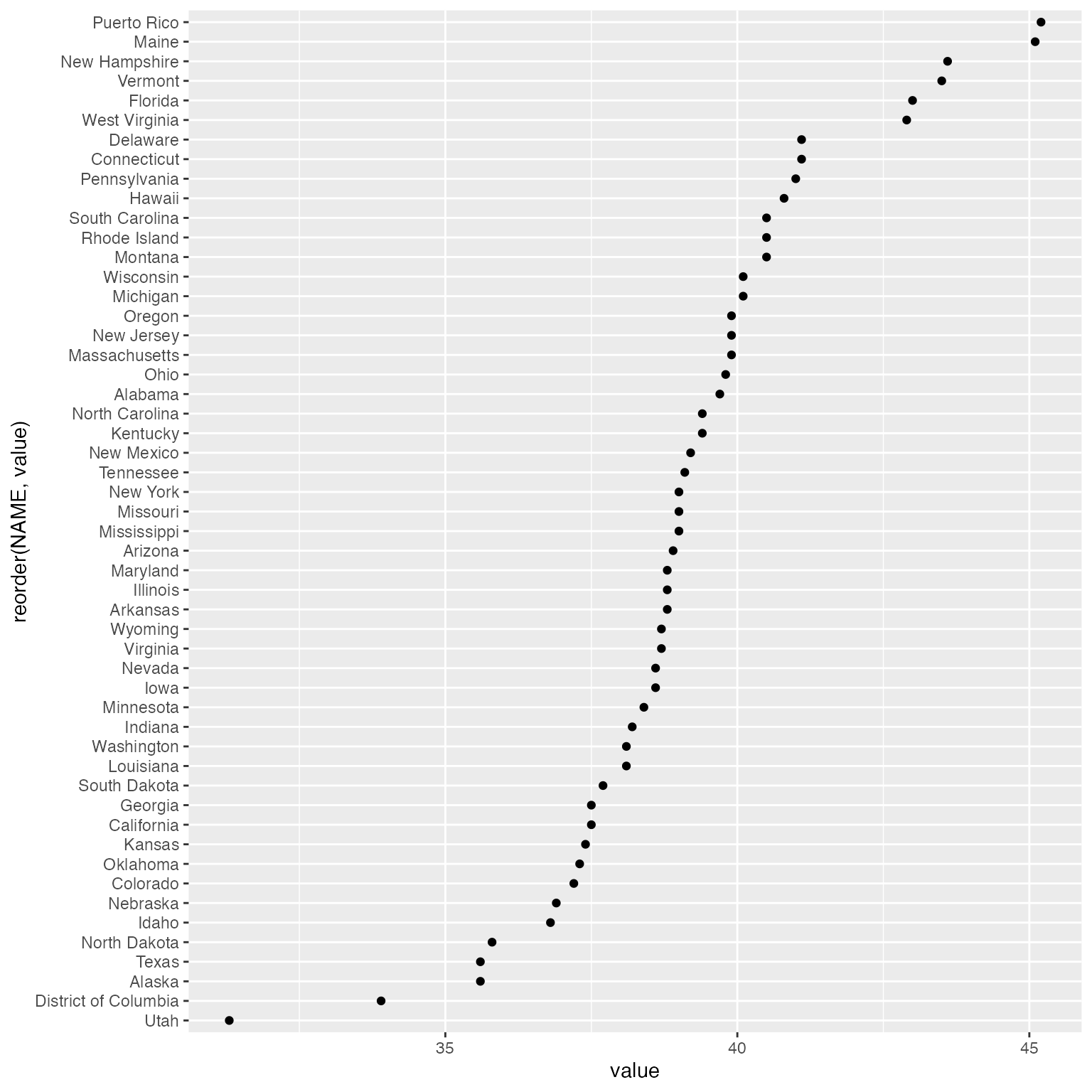
Geography in tidycensus
To get decennial Census data or American Community Survey data,
tidycensus users supply an argument to the required
geography parameter. Arguments are formatted as consumed by
the Census API, and specified in the table below. Not all geographies
are available for all surveys, all years, and all variables. Most Census
geographies are supported in tidycensus at the moment; if you require a
geography that is missing from the table below, please file an issue at
https://github.com/walkerke/tidycensus/issues.
If state or county is in bold face in “Available by”, you are required to supply a state and/or county for the given geography.
| Geography | Definition | Available by | Available in |
|---|---|---|---|
"us" |
United States |
get_acs(), get_decennial()
|
|
"region" |
Census region |
get_acs(), get_decennial()
|
|
"division" |
Census division |
get_acs(), get_decennial()
|
|
"state" |
State or equivalent | state |
get_acs(), get_decennial()
|
"county" |
County or equivalent | state, county |
get_acs(), get_decennial()
|
"county subdivision" |
County subdivision | state, county |
get_acs(), get_decennial()
|
"tract" |
Census tract | state, county |
get_acs(), get_decennial()
|
"block group" OR "cbg"
|
Census block group | state, county |
get_acs(), get_decennial()
|
"block" |
Census block | state, county | get_decennial() |
"place" |
Census-designated place | state |
get_acs(), get_decennial()
|
"alaska native regional corporation" |
Alaska native regional corporation | state |
get_acs(), get_decennial()
|
"american indian area/alaska native area/hawaiian home land" |
Federal and state-recognized American Indian reservations and Hawaiian home lands | state |
get_acs(), get_decennial()
|
"american indian area/alaska native area (reservation or statistical entity only)" |
Only reservations and statistical entities | state |
get_acs(), get_decennial()
|
"american indian area (off-reservation trust land only)/hawaiian home land" |
Only off-reservation trust lands and Hawaiian home lands | state | get_acs() |
"metropolitan/micropolitan statistical area" (2021
5-year ACS and later) OR
"metropolitan statistical area/micropolitan statistical area"
OR "cbsa"
|
Core-based statistical area |
get_acs(), get_decennial()
|
|
"combined statistical area" |
Combined statistical area | state |
get_acs(), get_decennial()
|
"new england city and town area" |
New England city/town area | state |
get_acs(), get_decennial()
|
"combined new england city and town area" |
Combined New England area | state |
get_acs(), get_decennial()
|
"urban area" |
Census-defined urbanized areas |
get_acs(), get_decennial()
|
|
"congressional district" |
Congressional district for the year-appropriate Congress | state |
get_acs(), get_decennial()
|
"school district (elementary)" |
Elementary school district | state |
get_acs(), get_decennial()
|
"school district (secondary)" |
Secondary school district | state |
get_acs(), get_decennial()
|
"school district (unified)" |
Unified school district | state |
get_acs(), get_decennial()
|
"public use microdata area" |
PUMA (geography associated with Census microdata samples) | state | get_acs() |
"zip code tabulation area" OR "zcta"
|
Zip code tabulation area |
get_acs(), get_decennial()
|
|
"state legislative district (upper chamber)" |
State senate districts | state |
get_acs(), get_decennial()
|
"state legislative district (lower chamber)" |
State house districts | state |
get_acs(), get_decennial()
|
"voting district" |
Voting districts (2020 only) | state | get_decennial() |
Searching for variables
Getting variables from the Census or ACS requires knowing the
variable ID - and there are thousands of these IDs across the different
Census files. To rapidly search for variables, use the
load_variables() function. The function takes two required
arguments: the year of the Census or endyear of the ACS sample, and the
dataset name, which varies in availability by year. For the decennial
Census, possible dataset choices include "pl" for the
redistricting files; "dhc", "dp",
"ddhca", "ddhcb", and "sdhc" for
the Demographic and Housing Characteristics, Demographic Profile,
Detailed DHC-A, Detailed DHC-B, and Supplemental DHC summary files (2020
only); and "sf1" or "sf2" (2000 and 2010) and
"sf3" or "sf4" (2000 only) for the legacy
summary files. Special island area summary files are available with
"as", "mp", "gu", or
"vi".
For the ACS, use either "acs1" or "acs5"
for the ACS detailed tables, and append /profile for the
Data Profile, /subject for the Subject Tables, or
/cprofile for the Comparison Profile. To browse these
variables, assign the result of this function to a variable and use the
View function in RStudio. An optional argument
cache = TRUE will cache the dataset on your computer for
future use.
v24 <- load_variables(2024, "acs5", cache = TRUE)

View(v24)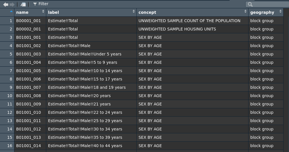
By filtering for “median age” variable IDs corresponding to that
query can be browsed interactively. For the 5-year ACS detailed tables
(denoted by "acs5"), a geography column will
also be returned that tells users the smallest geography at which a
given variable is available.
Working with ACS data
American Community Survey (ACS) data are available from the 1-year
ACS since 2005 for geographies of population 65,000 and greater, and
from the 5-year ACS for all geographies down to the block group level
starting with the 2005-2009 dataset. get_acs() defaults to
the 5-year ACS with the argument survey = "acs5", but
1-year ACS data are available using survey = "acs1".
ACS data differ from decennial Census data as they are based on an
annual sample of approximately 3 million households, rather than a more
complete enumeration of the US population. In turn, ACS data points are
estimates characterized by a margin of
error. tidycensus will always return the
estimate and margin of error together for any requested variables when
using get_acs(). In turn, when requesting ACS data with
tidycensus, it is not necessary to specify the
"E" or "M" suffix for a variable name. Let’s
fetch median household income data from the 2020-2024 ACS for counties
in Vermont.
vt <- get_acs(geography = "county",
              variables = c(medincome = "B19013_001"),
              state = "VT",
              year = 2024)

vt
## # A tibble: 14 × 5
## GEOID NAME variable estimate moe
## <chr> <chr> <chr> <dbl> <dbl>
## 1 50001 Addison County, Vermont medincome 89639 4396
## 2 50003 Bennington County, Vermont medincome 73325 4802
## 3 50005 Caledonia County, Vermont medincome 69970 5116
## 4 50007 Chittenden County, Vermont medincome 96759 3007
## 5 50009 Essex County, Vermont medincome 59294 3865
## 6 50011 Franklin County, Vermont medincome 81313 4757
## 7 50013 Grand Isle County, Vermont medincome 97396 12241
## 8 50015 Lamoille County, Vermont medincome 74908 6337
## 9 50017 Orange County, Vermont medincome 82232 4582
## 10 50019 Orleans County, Vermont medincome 70103 3179
## 11 50021 Rutland County, Vermont medincome 68616 2664
## 12 50023 Washington County, Vermont medincome 83449 2615
## 13 50025 Windham County, Vermont medincome 72217 4229
## 14 50027 Windsor County, Vermont medincome 77594 3244The output is similar to a call to get_decennial(), but
instead of a value column, get_acs returns
estimate and moe columns for the ACS estimate
and margin of error, respectively. moe represents the
default 90 percent confidence level around the estimate; this can be
changed to 95 or 99 percent with the moe_level parameter in
get_acs if desired.
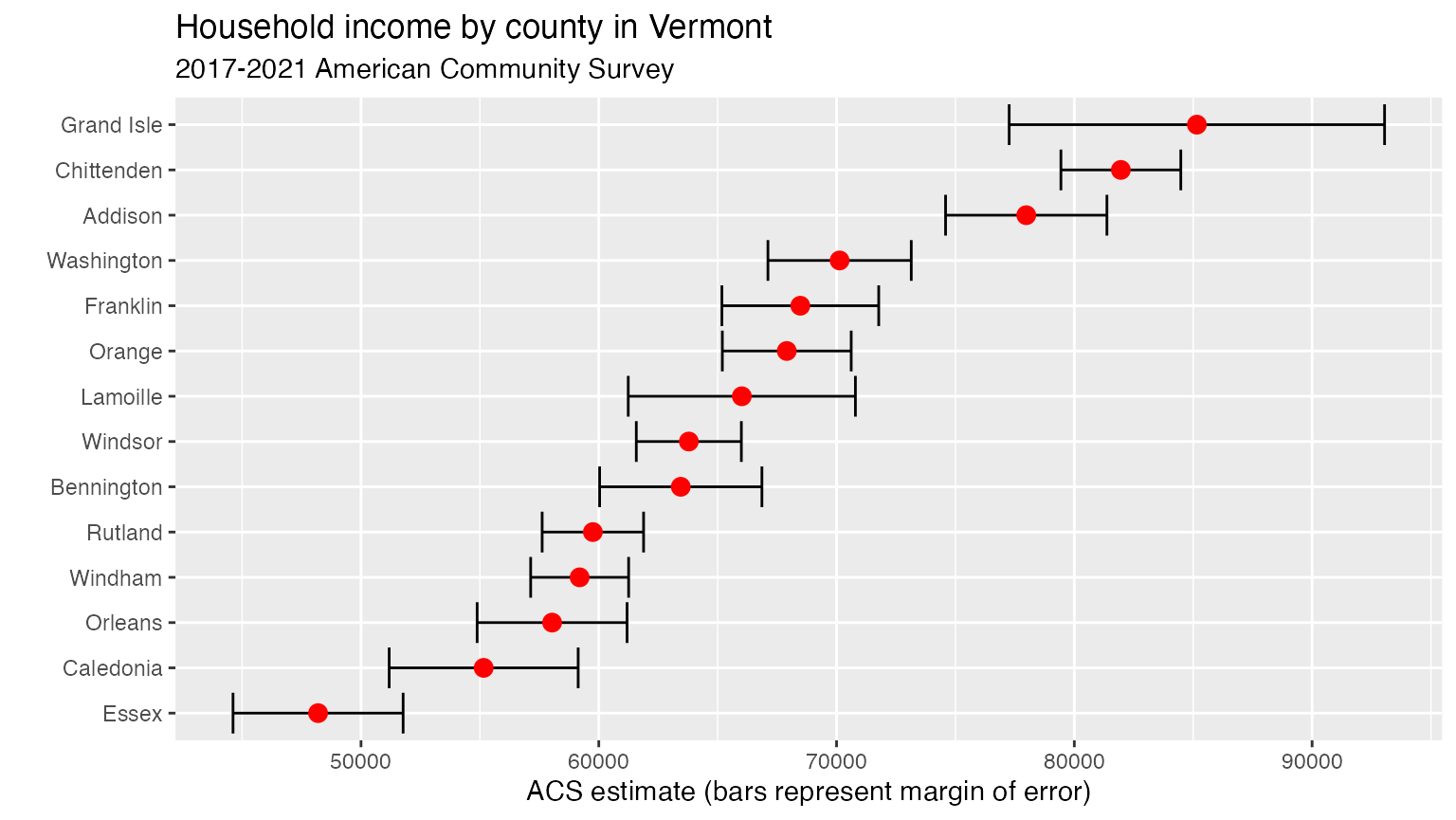
As we have the margin of error, we can visualize the uncertainty around the estimate:
vt |>
  mutate(NAME = gsub(" County, Vermont", "", NAME)) |>
  ggplot(aes(x = estimate, y = reorder(NAME, estimate))) +
  geom_errorbarh(aes(xmin = estimate - moe, xmax = estimate + moe)) +
  geom_point(color = "red", size = 3) +
  labs(title = "Household income by county in Vermont",
       subtitle = "2020-2024 American Community Survey",
       y = "",
       x = "ACS estimate (bars represent margin of error)")