Most of the data available through tidycensus and the Census API is
aggregated to certain geographic levels (tract, county, state, etc.). In
other words, the data we get by executing get_acs() has
been summarized by the Census Bureau so that we are able to learn how
many people live in a particular county or what the median household
income of a state is. There are thousands of individual variables that
the Census aggregates and publishes in tabular form.
For many purposes, these pre-aggregated tables have enough information to work with. But, the Census Bureau also releases microdata from the American Community Survey. Microdata is the individual-level responses to the ACS that is used to create the summary and detail tables the Census publishes. Instead of a getting one row per state from a table, we can get one row per respondent. For the American Community Survey, this data is called the Public Use Microdata Sample (PUMS).
Using PUMS data instead of the published tables can be a very powerful tool. It can, for instance, allow you to create custom estimates that aren’t available in pre-aggregated tables. You can also use microdata to fit models on individual-level data instead of modeling block groups or census tracts.
PUMS data is available through the Census Bureau’s web API, which tidycensus wraps so you can pull microdata directly into R. Raw PUMS files can also be downloaded from the Census Bureau FTP site if you need the full underlying CSV/SAS files.
PUMAs
One trade-off with using PUMS data as compared to aggregated data is that you only get the state and public use microdata area (PUMA) of each individual in the microdata. PUMAs are Census geographies that contain at least 100,000 people and are entirely within a single state. They are built from census tracts and counties and may or may not be similar to other recognized geographic boundaries. In New York City, for instance, PUMAs are closely aligned to Community Districts. So, if you are interested in pulling data about block groups, census tracts, or other small areas, you can’t use PUMS data.
PUMS data dictionaries
The first place to start is to identify the variables you want to
download. There are hundreds of PUMS variables and each describes
characteristics of a person or a housing unit.
pums_variables is a dataset built into tidycensus that
contains names, descriptions, codes, and other metadata about the PUMS
variables.
Because PUMS variables and codes can change slightly by year, you
should select which year’s data you will be working with and filter
pums_variables for only that year and survey. In the
following example, we will be working with the 2024 1-year American
Community Survey.
Later in this vignette, we use the survey and srvyr to calculate PUMS estimates, so if you want to follow along and you don’t already have them installed, you should install these two packages from CRAN.
install.packages(c("survey", "srvyr"))
library(tidyverse)
library(tidycensus)

pums_vars_2024 <- pums_variables |>
  filter(year == 2024, survey == "acs1")
pums_variables contains both the variables as well as
their possible values. So let’s just look at the unique variables.
pums_vars_2024 |>
  distinct(var_code, var_label, data_type, level)
## # A tibble: 520 × 4
## var_code var_label data_type level
## <chr> <chr> <chr> <chr>
## 1 SERIALNO Housing unit/GQ person serial number chr NA
## 2 DIVISION Division code based on 2020 Census definitions chr NA
## 3 PUMA Public use microdata area code (PUMA) based on 2020 Census definition (areas … chr NA
## 4 REGION Region code based on 2020 Census definitions chr NA
## 5 STATE State Code based on 2020 Census definitions chr NA
## # ℹ 515 more rowsIf you’re new to PUMS data, this is a good dataset to browse to get a feel for what variables are available.
Person vs. housing unit
Some PUMS variables relate to individuals (e.g. age, race, educational attainment) while others relate to households/housing units (e.g. number of bedrooms, electricity cost, property value).
Individuals in PUMS data are always nested within a housing unit (The
ACS is sent to an housing unit address and all people living in that
unit complete the survey.) Housing units are uniquely identified by the
SERIALNO variable and persons are uniquely identified by
the combination of SERIALNO and SPORDER. In
the data dictionary included in tidycensus, variables are identified as
either “housing” or “person” variables in the level column. Here, for
example, are the first five person-level variables in the data
dictionary.
## # A tibble: 279 × 4
##   var_code var_label                       data_type level
##   <chr>    <chr>                           <chr>     <chr>
## 1 SPORDER  Person number                   num       person
## 2 PWGTP    Person's weight                 num       person
## 3 AGEP     Age                             num       person
## 4 CIT      Citizenship status              chr       person
## 5 CITWP    Year of naturalization write-in num       person
## # ℹ 274 more rows
It is important to be mindful of whether the variables you choose to analyze are person- or household-level variables.
Using get_pums() to download PUMS data
To download PUMS data from the Census API, use the
get_pums() function. If you’ve used other
get_*() functions in tidycensus, it should be familiar to
you. The key arguments to specify are variables,
state, survey, and year. Here we
get PUMA, SEX, AGEP, and
SCHL variables for Vermont from the 2024 1-year ACS.
vt_pums <- get_pums(
  variables = c("PUMA", "SEX", "AGEP", "SCHL"),
  state = "VT",
  survey = "acs1",
  year = 2024
  )
vt_pums## # A tibble: 6,938 × 9
## SERIALNO SPORDER WGTP PWGTP AGEP PUMA STATE SCHL SEX
## <chr> <dbl> <dbl> <dbl> <dbl> <chr> <chr> <chr> <chr>
## 1 2024HU0433528 1 81 81 43 00200 50 23 1
## 2 2024HU0434577 1 67 66 41 00100 50 16 2
## 3 2024HU0434577 2 67 51 63 00100 50 17 1
## 4 2024HU0434839 1 36 36 64 00200 50 18 2
## 5 2024HU0435199 1 12 12 62 00400 50 16 1
## # ℹ 6,933 more rowsWe get 6938 rows and 9 columns. In addition to the variables we
specified, get_pums() also always returns
SERIALNO, SPORDER, WGTP,
PWGTP, and STATE. SERIALNO and
SPORDER are the variables that uniquely identify
observations, WGTP and PWGTP are the
housing-unit and person weights, and STATE is the state
code.
Notice that STATE, SEX and
SCHL return coded character variables. You can look up what
these codes represent in the pums_variables dataset
provided or set recode = TRUE in get_pums() to
return additional columns with the values of these variables
recoded.
vt_pums_recoded <- get_pums(
  variables = c("PUMA", "SEX", "AGEP", "SCHL"),
  state = "VT",
  survey = "acs1",
  year = 2024,
  recode = TRUE
  )
vt_pums_recoded## # A tibble: 6,938 × 12
## SERIALNO SPORDER WGTP PWGTP AGEP PUMA STATE SCHL SEX STATE_label SCHL_label SEX_label
## <chr> <dbl> <dbl> <dbl> <dbl> <chr> <chr> <chr> <chr> <ord> <ord> <ord>
## 1 2024GQ0000064 1 0 72 60 00400 50 18 2 Vermont/VT Some college, bu… Female
## 2 2024GQ0000879 1 0 13 20 00300 50 19 1 Vermont/VT 1 or more years … Male
## 3 2024GQ0001323 1 0 17 88 00300 50 13 1 Vermont/VT Grade 10 Male
## 4 2024GQ0001439 1 0 22 88 00200 50 16 2 Vermont/VT Regular high sch… Female
## 5 2024GQ0002242 1 0 60 41 00100 50 21 1 Vermont/VT Bachelor's degree Male
## # ℹ 6,933 more rowsAnalyzing PUMS data
Remember that PUMS data is a sample of about 1% of the US population. When we want to estimate a variable that represents the entire population rather than a sample, we have to apply a weighting adjustment. A simple way to think about PUMS weights is that for each observation in the sample, the weight variable tells us the number of people in the population that the observation represents. So, if we simply add up all the person weights in our VT PUMS data, we get the (estimated) population of Vermont.
sum(vt_pums_recoded$PWGTP)## [1] 648493Another convenient approach to weighting PUMS data is to use the
wt argument in dplyr::count(). Here, we
calculate the population by sex for each PUMA in Vermont (there are only
four in the whole state!).
vt_pums_recoded |>
  count(PUMA, SEX_label, wt = PWGTP)
## # A tibble: 8 × 3
## PUMA SEX_label n
## <chr> <ord> <dbl>
## 1 00100 Male 74417
## 2 00100 Female 74460
## 3 00200 Male 63202
## 4 00200 Female 64294
## 5 00300 Male 81955
## 6 00300 Female 89186
## 7 00400 Male 98563
## 8 00400 Female 102416Many of the variables included in the PUMS data are categorical and we might want to group some categories together and estimate the proportion of the population with these characteristics. In this example, we first create a new variable that is whether or not the person has a Bachelor’s degree or above, group by PUMA and sex, then calculate the total population, average age, total with BA or above (only for people 25 and older), and percent with BA or above.
vt_pums_recoded |>
  mutate(ba_above = SCHL %in% c("21", "22", "23", "24")) |>
  group_by(PUMA, SEX_label) |>
  summarize(
    total_pop = sum(PWGTP),
    mean_age = weighted.mean(AGEP, PWGTP),
    ba_above = sum(PWGTP[ba_above == TRUE & AGEP >= 25]),
    ba_above_pct = ba_above / sum(PWGTP[AGEP >= 25])
  )
## # A tibble: 8 × 6
## # Groups: PUMA [4]
## PUMA SEX_label total_pop mean_age ba_above ba_above_pct
## <chr> <ord> <dbl> <dbl> <dbl> <dbl>
## 1 00100 Male 74417 42.7 18107 0.329
## 2 00100 Female 74460 43.5 24192 0.435
## 3 00200 Male 63202 43.2 20504 0.434
## 4 00200 Female 64294 45.3 26691 0.540
## 5 00300 Male 81955 39.2 32670 0.590
## 6 00300 Female 89186 40.0 35898 0.603
## 7 00400 Male 98563 44.8 30702 0.419
## 8 00400 Female 102416 46.6 35577 0.453Calculating standard errors
In the previous examples, you might have noticed that we calculate a point estimate, but do not get a standard error or margin of error as is included in aggregated Census tables. It is important to calculate standard errors when making custom estimates using PUMS data, because it can be easy to create a very small sub-group where there are not enough observations in the sample to make a reliable estimate.
The standard package for calculating estimates and fitting models
with complex survey objects is the survey
package. The srvyr
package is an alternative and wraps some survey functions to allow
for analyzing surveys using dplyr-style syntax.
tidycensus provides a function, to_survey(), that converts
data frames returned by get_pums() into either a survey or
srvyr object.
In order to generate reliable standard errors, the Census Bureau provides a set of replicate weights for each observation in the PUMS dataset. These replicate weights are used to simulate multiple samples from the single PUMS sample and can be used to calculate more precise standard errors. PUMS data contains both person- and housing-unit-level replicate weights.
To download replicate weights along with PUMS data, set the
rep_weights argument in get_pums() to
"person", "housing", or "both".
Here we get the same Vermont PUMS data as above in addition to the 80
person replicate weight columns.
vt_pums_rep_weights <- get_pums(
  variables = c("PUMA", "SEX", "AGEP", "SCHL"),
  state = "VT",
  survey = "acs1",
  year = 2024,
  recode = TRUE,
  rep_weights = "person"
  )
To easily convert this data frame to a survey or srvyr object, we can
use the to_survey() function.
vt_survey_design <- to_survey(vt_pums_rep_weights)By default, to_survey() converts a data frame to a
tbl_svy object by using person replicate weights. You can
change the arguments in to_survey if you are analyzing
housing-unit data (type = "housing") or if you want a
survey object instead of a srvyr object. (Although, tbl_svy
objects also have a svyrep.design class so you can use
survey functions on srvyr objects.)
Now, with our srvyr design object defined, we can calculate the same estimates as above, but we now get column with standard errors as well.
library(srvyr, warn.conflicts = FALSE)

vt_survey_design |>
  survey_count(PUMA, SEX_label)
## # A tibble: 8 × 4
## PUMA SEX_label n n_se
## <chr> <ord> <dbl> <dbl>
## 1 00100 Male 74417 655.
## 2 00100 Female 74460 654.
## 3 00200 Male 63202 501.
## 4 00200 Female 64294 502.
## 5 00300 Male 81955 891.
## 6 00300 Female 89186 1009.
## 7 00400 Male 98563 745.
## 8 00400 Female 102416 783.The srvyr syntax is very similar to standard dplyr syntax, so this
should look familiar; we’ve swapped out count() for
survey_count() and we don’t need a wt argument
because we defined the weights when we set up the srvyr object.
The equivalent estimate using survey syntax looks like this:
##        PUMA SEX_labelMale SEX_labelFemale      se1       se2
## 00100 00100         74417           74460 655.2191  653.8106
## 00200 00200         63202           64294 501.2731  501.9494
## 00300 00300         81955           89186 891.1254 1008.5331
## 00400 00400         98563          102416 744.7937  782.8687
We can also repeat the estimate we did above and calculate the percentage of people that are 25 and up with a bachelor’s degree, while this time returning the upper and lower bounds of the confidence interval for these estimates. This time though, we have to subset our data frame to only those 25 and older before we summarize.
vt_survey_design |>
  mutate(ba_above = SCHL %in% c("21", "22", "23", "24")) |>
  filter(AGEP >= 25) |>
  group_by(PUMA, SEX_label) |>
  summarize(
    age_25_up = survey_total(vartype = "ci"),
    ba_above_n = survey_total(ba_above, vartype = "ci"),
    ba_above_pct = survey_mean(ba_above, vartype = "ci")
    )
## # A tibble: 8 × 11
## # Groups: PUMA [4]
## PUMA SEX_label age_25_up age_25_up_low age_25_up_upp ba_above_n ba_above_n_low ba_above_n_upp
## <chr> <ord> <dbl> <dbl> <dbl> <dbl> <dbl> <dbl>
## 1 00100 Male 55021 53760. 56282. 18107 15532. 20682.
## 2 00100 Female 55648 54783. 56513. 24192 20869. 27515.
## 3 00200 Male 47190 46035. 48345. 20504 17395. 23613.
## 4 00200 Female 49422 48426. 50418. 26691 23703. 29679.
## 5 00300 Male 55363 54108. 56618. 32670 28820. 36520.
## 6 00300 Female 59502 58048. 60956. 35898 32411. 39385.
## 7 00400 Male 73203 71956. 74450. 30702 27518. 33886.
## 8 00400 Female 78520 76927. 80113. 35577 32370. 38784.
## # ℹ 3 more variables: ba_above_pct <dbl>, ba_above_pct_low <dbl>, ba_above_pct_upp <dbl>Modeling with PUMS data
An important use case for PUMS data is doing regression analysis or
other modeling. Let’s try to predict the length of an individual’s
commute to work (JWMNP) based on their wages, employer type
(private, public, self), and which PUMA they live in. We’ll use
Massachusetts and the 2020-2024 5-year estimates — Massachusetts has
dozens of PUMAs, which gives PUMA more variation as a
categorical predictor than a small state would.
The 5-year PUMS file for Massachusetts is a sizable download, so we cache it locally after the first pull to keep subsequent vignette rebuilds quick:
cache_file <- "cache/ma_pums_to_model.rds"

if (file.exists(cache_file)) {
  ma_pums_to_model <- readRDS(cache_file)
} else {
  ma_pums_to_model <- get_pums(
    variables = c("PUMA", "WAGP", "JWMNP", "JWTRNS", "COW", "ESR"),
    state = "MA",
    survey = "acs5",
    year = 2024,
    rep_weights = "person"
    )
  dir.create("cache", showWarnings = FALSE)
  saveRDS(ma_pums_to_model, cache_file)
}
Now, we filter out observations that aren’t relevant, do a little
recoding of the class of worker variable, and finally convert the data
frame to a survey design object. Note that the
means-of-transportation-to-work variable was renamed from
JWTR to JWTRNS starting with the 2019 ACS,
though code 11 (“Worked from home”) is unchanged.
ma_model_sd <- ma_pums_to_model |>
  filter(
    ESR == 1,     # civilian employed
    JWTRNS != 11, # does not work at home
    WAGP > 0,     # earned wages last year
    JWMNP > 0     # commute more than zero min
    ) |>
  mutate(
    emp_type = case_when(
      COW %in% c("1", "2")      ~ "private",
      COW %in% c("3", "4", "5") ~ "public",
      TRUE                      ~ "self"
      )
    ) |>
  to_survey()
Let’s quickly check out some summary stats using
srvyr.
ma_model_sd |>
  summarize(
    n              = survey_total(1),
    mean_wage      = survey_mean(WAGP),
    median_wage    = survey_median(WAGP),
    mean_commute   = survey_mean(JWMNP),
    median_commute = survey_median(JWMNP)
    )
## # A tibble: 1 × 10
## n n_se mean_wage mean_wage_se median_wage median_wage_se mean_commute mean_commute_se
## <dbl> <dbl> <dbl> <dbl> <dbl> <dbl> <dbl> <dbl>
## 1 2821931 6477. 72065. 257. 52000 251. 29.1 0.0876
## # ℹ 2 more variables: median_commute <dbl>, median_commute_se <dbl>
ma_model_sd |>
  survey_count(emp_type)
## # A tibble: 3 × 3
## emp_type n n_se
## <chr> <dbl> <dbl>
## 1 private 2303786 7464.
## 2 public 406418 3504.
## 3 self 111727 1945.And now we’re ready to fit a simple linear regression model.
model <- survey::svyglm(log(JWMNP) ~ log(WAGP) + emp_type + PUMA, design = ma_model_sd)
summary(model)
##
## Call:
## survey::svyglm(formula = log(JWMNP) ~ log(WAGP) + emp_type +
## PUMA, design = ma_model_sd)
##
## Survey design:
## Called via srvyr
##
## Coefficients:
## Estimate Std. Error t value Pr(>|t|)
## (Intercept) 1.469027 0.034781 42.236 < 2e-16 ***
## log(WAGP) 0.121455 0.002462 49.328 < 2e-16 ***
## emp_typepublic -0.125827 0.007878 -15.972 6.09e-14 ***
## emp_typeself -0.160817 0.017392 -9.247 3.28e-09 ***
## PUMA00201 0.232164 0.031614 7.344 1.80e-07 ***
## PUMA00301 0.107476 0.032507 3.306 0.003084 **
## PUMA00401 0.161824 0.025371 6.378 1.65e-06 ***
## PUMA00402 0.079145 0.031614 2.503 0.019842 *
## PUMA00403 0.190539 0.029714 6.412 1.52e-06 ***
## PUMA00501 0.365703 0.032791 11.152 9.40e-11 ***
## PUMA00502 0.286255 0.032049 8.932 6.16e-09 ***
## PUMA00503 0.381410 0.029028 13.139 3.54e-12 ***
## PUMA00504 0.143294 0.033677 4.255 0.000298 ***
## PUMA00505 0.166017 0.033571 4.945 5.34e-05 ***
## PUMA00506 0.372555 0.029273 12.727 6.77e-12 ***
## PUMA00507 0.402752 0.028577 14.094 8.38e-13 ***
## PUMA00601 0.414236 0.028101 14.741 3.29e-13 ***
## PUMA00602 0.365396 0.027895 13.099 3.77e-12 ***
## PUMA00603 0.348078 0.024136 14.422 5.20e-13 ***
## PUMA00604 0.440808 0.029864 14.760 3.20e-13 ***
## PUMA00605 0.381296 0.033133 11.508 5.07e-11 ***
## PUMA00606 0.424064 0.032362 13.104 3.74e-12 ***
## PUMA00607 0.301536 0.029415 10.251 4.78e-10 ***
## PUMA00608 0.351882 0.028843 12.200 1.59e-11 ***
## PUMA00609 0.511471 0.027684 18.475 2.70e-15 ***
## PUMA00610 0.500293 0.031016 16.130 4.95e-14 ***
## PUMA00611 0.266214 0.025096 10.608 2.48e-10 ***
## PUMA00612 0.390724 0.028201 13.855 1.19e-12 ***
## PUMA00613 0.266217 0.026001 10.239 4.89e-10 ***
## PUMA00701 0.290667 0.030754 9.451 2.19e-09 ***
## PUMA00702 0.219829 0.030629 7.177 2.62e-07 ***
## PUMA00703 0.347840 0.032720 10.631 2.38e-10 ***
## PUMA00704 0.314478 0.027598 11.395 6.16e-11 ***
## PUMA00705 0.475151 0.029555 16.077 5.31e-14 ***
## PUMA00706 0.303491 0.028110 10.797 1.77e-10 ***
## PUMA00801 0.394437 0.030328 13.006 4.36e-12 ***
## PUMA00802 0.303524 0.028253 10.743 1.94e-10 ***
## PUMA00803 0.486241 0.028806 16.880 1.88e-14 ***
## PUMA00804 0.573424 0.028076 20.424 3.06e-16 ***
## PUMA00805 0.524450 0.031961 16.409 3.44e-14 ***
## PUMA00806 0.521434 0.032907 15.846 7.21e-14 ***
## PUMA00901 0.330769 0.031195 10.603 2.50e-10 ***
## PUMA00902 0.362824 0.033241 10.915 1.43e-10 ***
## PUMA00903 0.583113 0.030691 18.999 1.48e-15 ***
## PUMA00904 0.523385 0.029719 17.611 7.59e-15 ***
## PUMA00905 0.488854 0.030662 15.943 6.33e-14 ***
## PUMA00906 0.451395 0.029828 15.133 1.90e-13 ***
## PUMA01001 0.385390 0.028835 13.365 2.50e-12 ***
## PUMA01002 0.408159 0.029473 13.848 1.20e-12 ***
## PUMA01003 0.264311 0.032432 8.150 3.12e-08 ***
## PUMA01004 0.228814 0.025499 8.974 5.66e-09 ***
## PUMA01101 0.444206 0.032848 13.523 1.97e-12 ***
## PUMA01102 0.413555 0.035251 11.732 3.47e-11 ***
## PUMA01103 0.438164 0.029366 14.921 2.56e-13 ***
## PUMA01104 0.405079 0.026141 15.496 1.15e-13 ***
## PUMA01201 0.142114 0.029368 4.839 6.96e-05 ***
## PUMA01301 -0.078390 0.039338 -1.993 0.058291 .
## ---
## Signif. codes: 0 '***' 0.001 '**' 0.01 '*' 0.05 '.' 0.1 ' ' 1
##
## (Dispersion parameter for gaussian family taken to be 0.6160352)
##
## Number of Fisher Scoring iterations: 2Notice that the PUMA dummies are almost all positive — commute times
are dominated by the Boston-area job-shed PUMAs, where workers travel
farther into the regional employment core. (The reference level here is
whichever PUMA code is first when R coerces PUMA to a
factor; the substantive takeaway is the relative pattern across PUMAs,
not the specific reference.)
Mapping PUMS data
If you’ve used the spatial functionality in tidycensus before, you
might also want to put your custom PUMS estimates on a map. To do this,
let’s use tigris to download PUMA boundaries for the states
in New England as an sf object. ACS data from 2022 onward
use the 2020-vintage PUMA boundaries, so we request those:
ne_states <- c("VT", "NH", "ME", "MA", "CT", "RI")
ne_pumas <- map(ne_states, tigris::pumas, class = "sf", cb = TRUE, year = 2020) |>
  reduce(rbind)
Next we download the income-to-poverty ratio from the PUMS dataset and calculate the percentage of population below 200% of the poverty line for each PUMA.
ne_pums <- get_pums(
  variables = c("PUMA", "POVPIP"),
  state = ne_states,
  survey = "acs1",
  year = 2024
  )

ne_pov <- ne_pums |>
  group_by(STATE, PUMA) |>
  summarize(
    total_pop = sum(PWGTP),
    pct_in_pov = sum(PWGTP[POVPIP < 200]) / total_pop
  )
And now we can make a choropleth map by joining the PUMA boundaries with the PUMS data.
ne_pumas |>
  left_join(ne_pov, by = c("STATEFP20" = "STATE", "PUMACE20" = "PUMA")) |>
  ggplot(aes(fill = pct_in_pov)) +
  geom_sf() +
  scale_fill_viridis_b(
    name = NULL,
    option = "magma",
    labels = scales::label_percent(1)
    ) +
  labs(title = "Percentage of population below 200% of the poverty line") +
  theme_void()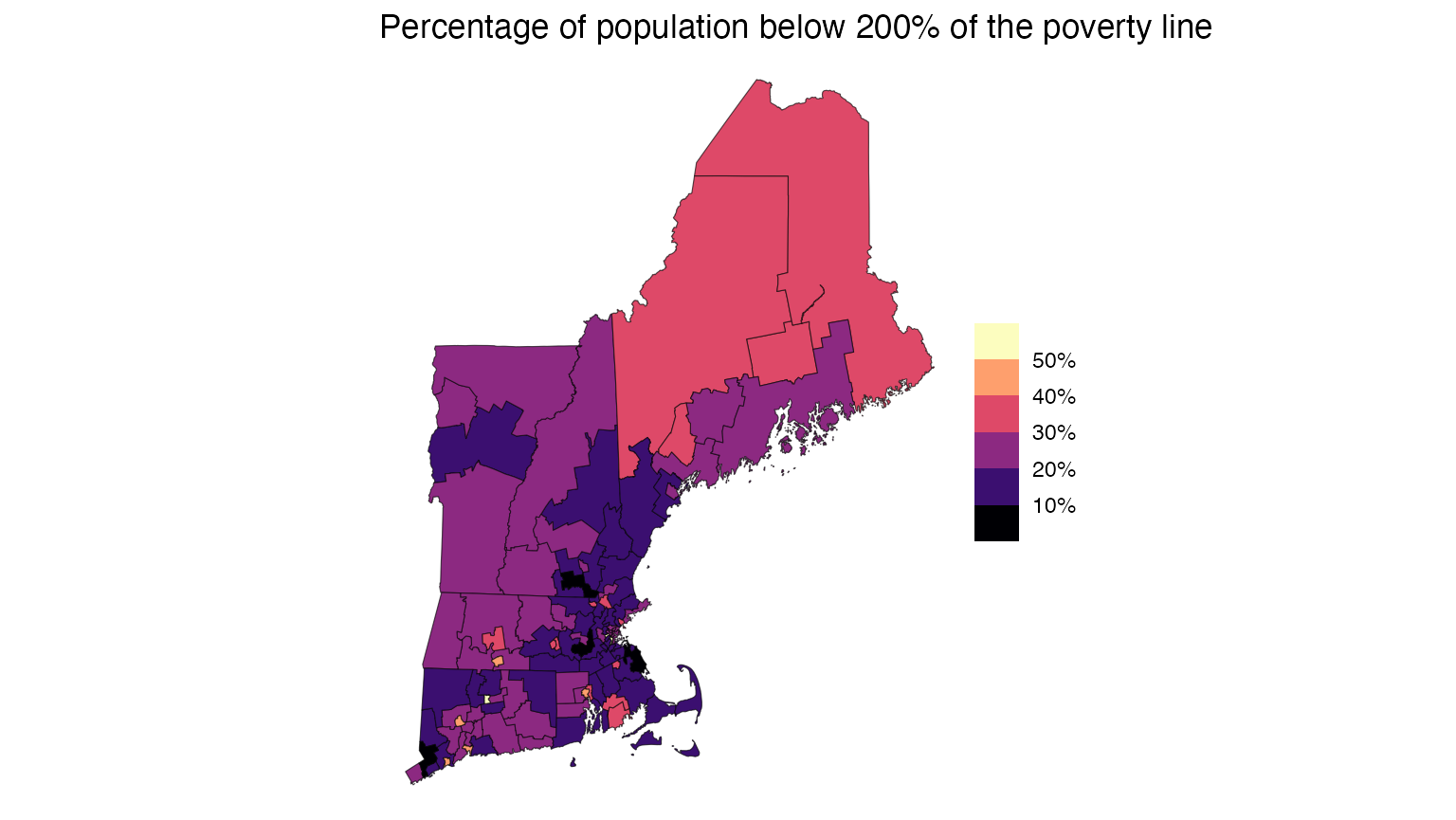
Verification of PUMS estimates
The Census Bureau publishes calculated estimates and standard errors for a number of states and variables in a year-specific user verification file, so that users can confirm their PUMS analysis matches the expected values.
Here are a few estimates we’ll verify from the 2024 ACS 1-year PUMS
user verification file. Note that the household-relationship variable
was renamed from RELP to RELSHIPP starting
with the 2019 ACS, and the institutionalized group quarters category is
now RELSHIPP = 37 (previously RELP = 16):
| State | Variable | Estimate | SE |
|---|---|---|---|
| Wyoming | GQ institutional population (RELSHIPP = 37) | 6504 | 3 |
| Utah | Owned free and clear (TEN = 2) | 264934 | 4503 |
| Hawaii | Age 0-4 | 77096 | 1182 |
wy_relshipp <- get_pums(
  variables = "RELSHIPP",
  state = "Wyoming",
  survey = "acs1",
  year = 2024,
  rep_weights = "person"
)

ut_ten <- get_pums(
  variables = "TEN",
  state = "Utah",
  survey = "acs1",
  year = 2024,
  rep_weights = "housing"
)

hi_age <- get_pums(
  variables = "AGEP",
  state = "Hawaii",
  survey = "acs1",
  year = 2024,
  rep_weights = "person"
)
wy_relshipp |>
  to_survey() |>
  survey_count(RELSHIPP) |>
  filter(RELSHIPP == "37")
## # A tibble: 1 × 3
## RELSHIPP n n_se
## <chr> <dbl> <dbl>
## 1 37 6504 2.93
ut_ten |>
  distinct(SERIALNO, .keep_all = TRUE) |>
  to_survey(type = "housing") |>
  survey_count(TEN) |>
  filter(TEN == 2)
## # A tibble: 1 × 3
## TEN n n_se
## <chr> <dbl> <dbl>
## 1 2 264934 4503.
hi_age |>
  filter(between(AGEP, 0, 4)) |>
  to_survey() |>
  summarize(age_0_4 = survey_total(1))
## # A tibble: 1 × 2
## age_0_4 age_0_4_se
## <dbl> <dbl>
## 1 77096 1182.3 for 3 – yay!