The main intent of the tidycensus package is to return population characteristics of the United States in tidy format allowing for integration with simple feature geometries. Its intent is not, and has never been, to wrap the universe of APIs and datasets available from the US Census Bureau. For datasets not included in tidycensus, I recommend Hannah Recht’s censusapi package (https://github.com/hrecht/censusapi), which allows R users to access all Census APIs, and packages such as Jamaal Green’s lehdr package (https://github.com/jamgreen/lehdr) which grants R users access to Census Bureau LODES data.
However, tidycensus incorporates a select number of Census Bureau datasets outside the decennial Census and ACS that are aligned with the basic goals of the package. One such dataset is the Population Estimates API, which includes information on a wide variety of population characteristics that is updated annually. Also available through tidycensus is the Migration Flows API, which estimates the number of people that have moved between pairs of places in a given year.
Population estimates
Population estimates are available in tidycensus through the
get_estimates() function. Estimates are organized into
products, which in tidycensus include
"population", "components",
"housing", and "characteristics". The
population and housing products contain population/density and housing
unit estimates, respectively. The components of change and
characteristics products, in contrast, include a wider range of possible
variables.
The post-2020 Population Estimates are no longer on the Census API, but they are downloadable and usable in tidycensus. Follow the guide below for some examples.
Components of change population estimates
By default, specifying "population",
"components", or "housing" (housing is not
available for 2020 and later) as the product in
get_estimates() returns all variables associated with that
component. For example, we can request all components of change
variables for US states in 2024:
library(tidycensus)
library(tidyverse)
library(tigris)
options(tigris_use_cache = TRUE)

us_components <- get_estimates(geography = "state", product = "components", vintage = 2024)

us_components
## # A tibble: 676 × 5
## GEOID NAME variable year value
## <chr> <chr> <chr> <int> <dbl>
## 1 01 Alabama BIRTHS 2024 57541
## 2 01 Alabama DEATHS 2024 59273
## 3 01 Alabama NATURALCHG 2024 -1732
## 4 01 Alabama INTERNATIONALMIG 2024 15763
## 5 01 Alabama DOMESTICMIG 2024 26028
## 6 01 Alabama NETMIG 2024 41791
## 7 01 Alabama RESIDUAL 2024 -33
## 8 01 Alabama RBIRTH 2024 11.2
## 9 01 Alabama RDEATH 2024 11.5
## 10 01 Alabama RNATURALCHG 2024 -0.337
## # ℹ 666 more rowsThe variables included in the components of change product consist of
both estimates of counts and rates. Rates are preceded
by an R in the variable name and are calculated per 1000
residents.
unique(us_components$variable)## [1] "BIRTHS" "DEATHS" "NATURALCHG"
## [4] "INTERNATIONALMIG" "DOMESTICMIG" "NETMIG"
## [7] "RESIDUAL" "RBIRTH" "RDEATH"
## [10] "RNATURALCHG" "RINTERNATIONALMIG" "RDOMESTICMIG"
## [13] "RNETMIG"Available geographies include "us",
"state", "county",
"metropolitan statistical area/micropolitan statistical area"
or "cbsa", "combined statistical area", and
"place".
If desired, users can request a specific component or components by
supplying a character vector to the variables parameter, as
in other tidycensus functions. get_estimates() also
supports simple feature geometry integration to facilitate mapping. In
the example below, we’ll acquire data on the net migration rate between
2023 and 2024 for all counties in the United States. We’ll also use the
shift_geometry() function from the tigris
package to shift and rescale counties outside the continental US for
national mapping.
net_migration <- get_estimates(geography = "county",
                               variables = "RNETMIG",
                               vintage = 2024,
                               geometry = TRUE,
                               resolution = "20m") |>
  shift_geometry()

net_migration
## Simple feature collection with 3144 features and 5 fields
## Geometry type: GEOMETRY
## Dimension: XY
## Bounding box: xmin: -3112200 ymin: -1697728 xmax: 2258154 ymax: 1558935
## Projected CRS: USA_Contiguous_Albers_Equal_Area_Conic
## # A tibble: 3,144 × 6
## GEOID NAME variable year value geometry
## <chr> <chr> <chr> <int> <dbl> <MULTIPOLYGON [m]>
## 1 18087 LaGrange County, Indi… RNETMIG 2024 -6.33 (((851901.1 523582.1, 88…
## 2 20107 Linn County, Kansas RNETMIG 2024 -0.710 (((80824.31 100142.8, 12…
## 3 24029 Kent County, Maryland RNETMIG 2024 9.64 (((1676654 359059.5, 167…
## 4 31065 Furnas County, Nebras… RNETMIG 2024 -20.6 (((-353382.3 327213.1, -…
## 5 13237 Putnam County, Georgia RNETMIG 2024 13.8 (((1148068 -379579.8, 11…
## 6 20183 Smith County, Kansas RNETMIG 2024 10.7 (((-259486.4 284619.1, -…
## 7 08005 Arapahoe County, Colo… RNETMIG 2024 3.14 (((-758510 283522.7, -75…
## 8 05037 Cross County, Arkansas RNETMIG 2024 -9.92 (((446726.3 -228681.3, 4…
## 9 17009 Brown County, Illinois RNETMIG 2024 -0.793 (((429604 303394.6, 4479…
## 10 21061 Edmonson County, Kent… RNETMIG 2024 17.1 (((835236.9 21869.21, 85…
## # ℹ 3,134 more rowsWe’ll next use tidyverse tools to generate a groups
column that bins the net migration rates into comprehensible categories,
and plot the result using geom_sf() and ggplot2.
library(showtext)
font_add_google("Roboto")
showtext_auto()

order = c("-15 and below", "-15 to -5", "-5 to +5", "+5 to +15", "+15 and up")

net_migration <- net_migration |>
  mutate(groups = case_when(
    value > 15 ~ "+15 and up",
    value > 5 ~ "+5 to +15",
    value > -5 ~ "-5 to +5",
    value > -15 ~ "-15 to -5",
    TRUE ~ "-15 and below"
  )) |>
  mutate(groups = factor(groups, levels = order))

state_overlay <- states(
  cb = TRUE,
  resolution = "20m"
) |>
  filter(GEOID != "72") |>
  shift_geometry()

ggplot() +
  geom_sf(data = net_migration, aes(fill = groups, color = groups), size = 0.1) +
  geom_sf(data = state_overlay, fill = NA, color = "black", size = 0.1) +
  scale_fill_brewer(palette = "PuOr", direction = -1) +
  scale_color_brewer(palette = "PuOr", direction = -1, guide = FALSE) +
  coord_sf(datum = NA) +
  theme_minimal(base_family = "Roboto", base_size = 18) +
  labs(title = "Net migration per 1000 residents by county",
       subtitle = "US Census Bureau 2024 Population Estimates",
       fill = "Rate",
       caption = "Data acquired with the R tidycensus package | @kyle_e_walker")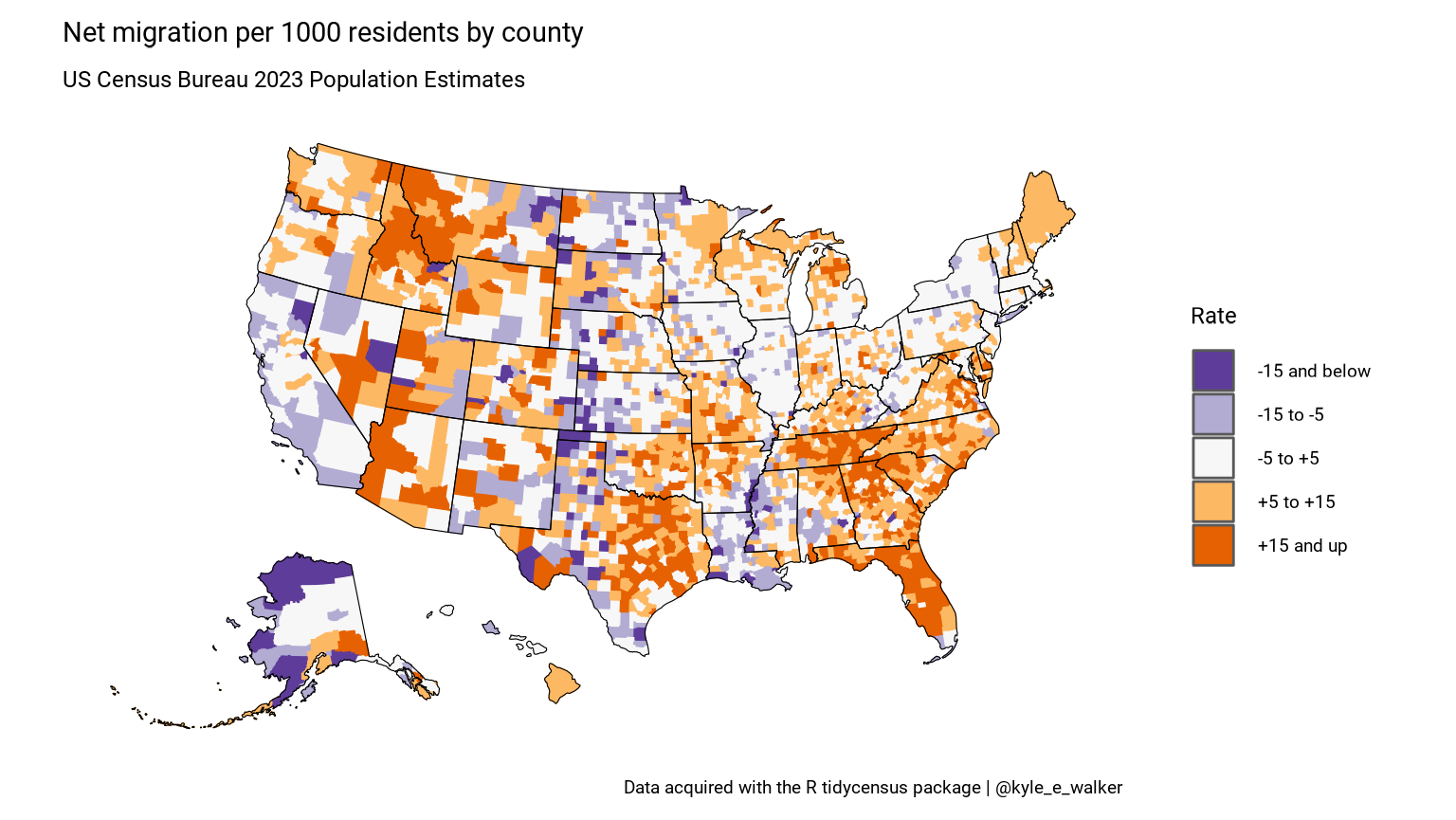
Estimates of population characteristics
The fourth population estimates product available in
get_estimates(), "characteristics", is
formatted differently than the other three. It returns population
estimates broken down by categories of AGEGROUP,
SEX, RACE, and HISP, for Hispanic
origin. Requested breakdowns should be specified as a character vector
supplied to the breakdown parameter when the
product is set to "characteristics".
By default, the returned categories are formatted as integers that
map onto the Census Bureau definitions explained here: https://www.census.gov/data/developers/data-sets/popest-popproj/popest/popest-vars/2017.html.
However, by specifying breakdown_labels = TRUE, the
function will return the appropriate labels instead. For example:
la_age_hisp <- get_estimates(geography = "county",
                             product = "characteristics",
                             breakdown = c("SEX", "AGEGROUP", "HISP"),
                             breakdown_labels = TRUE,
                             state = "CA",
                             county = "Los Angeles",
                             vintage = 2024)

la_age_hisp
## # A tibble: 114 × 7
## GEOID NAME year SEX AGEGROUP HISP value
## <chr> <chr> <dbl> <chr> <fct> <chr> <dbl>
## 1 06037 Los Angeles County, California 2024 Male All ages Both… 4.83e6
## 2 06037 Los Angeles County, California 2024 Male All ages Non-… 2.45e6
## 3 06037 Los Angeles County, California 2024 Male All ages Hisp… 2.38e6
## 4 06037 Los Angeles County, California 2024 Male Age 0 to 4 yea… Both… 2.43e5
## 5 06037 Los Angeles County, California 2024 Male Age 0 to 4 yea… Non-… 1.00e5
## 6 06037 Los Angeles County, California 2024 Male Age 0 to 4 yea… Hisp… 1.43e5
## 7 06037 Los Angeles County, California 2024 Male Age 5 to 9 yea… Both… 2.73e5
## 8 06037 Los Angeles County, California 2024 Male Age 5 to 9 yea… Non-… 1.18e5
## 9 06037 Los Angeles County, California 2024 Male Age 5 to 9 yea… Hisp… 1.55e5
## 10 06037 Los Angeles County, California 2024 Male Age 10 to 14 y… Both… 2.92e5
## # ℹ 104 more rowsWith some additional data wrangling, the returned format facilitates analysis and visualization. For example, we can compare population pyramids for Hispanic and non-Hispanic populations in Los Angeles County:
compare <- filter(la_age_hisp, str_detect(AGEGROUP, "^Age"),
                  HISP != "Both Hispanic Origins",
                  SEX != "Both sexes") |>
  mutate(value = ifelse(SEX == "Male", -value, value))

ggplot(compare, aes(x = AGEGROUP, y = value, fill = SEX)) +
  geom_bar(stat = "identity", width = 1) +
  theme_minimal(base_family = "Roboto") +
  scale_y_continuous(labels = function(y) paste0(abs(y / 1000), "k")) +
  scale_x_discrete(labels = function(x) gsub("Age | years", "", x)) +
  scale_fill_manual(values = c("darkred", "navy")) +
  coord_flip() +
  facet_wrap(~HISP) +
  labs(x = "",
       y = "2024 Census Bureau population estimate",
       title = "Population structure by Hispanic origin",
       subtitle = "Los Angeles County, California",
       fill = "",
       caption = "Data source: US Census Bureau population estimates & tidycensus R package")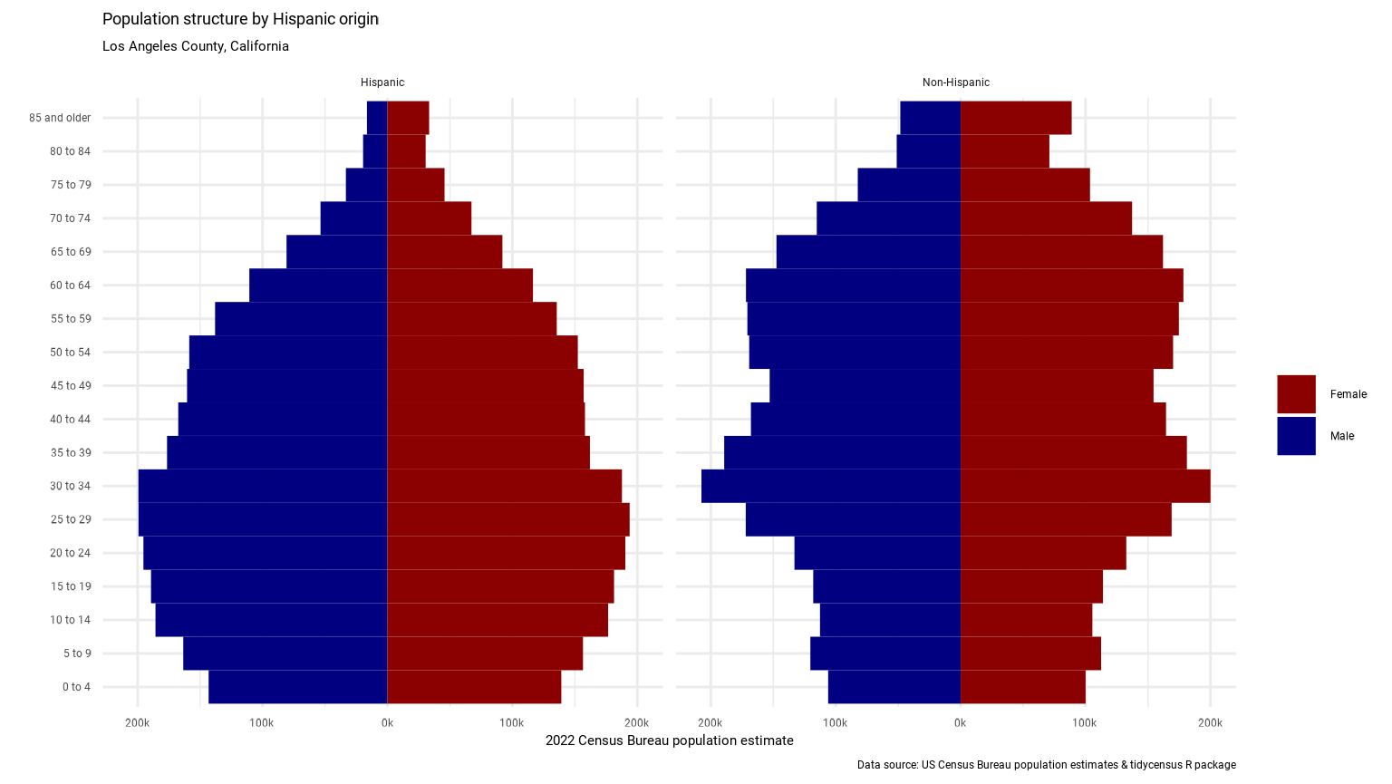
Migration flows
The American Community Survey Migration Flows dataset estimates the number of people that have moved between pairs of places. The estimates are calculated based on where a person lived when surveyed and where they lived one year prior to being surveyed. The data is available at three geographic levels: county, county subdivision (minor civil division), and metropolitan statistical area (MSA). Because the number of movers may be small for some pairs of counties, the data is aggregated over a five-year period. The estimates for each five-year period represent the number of people that moved between places each year during that period.
The data is set up such that for each county, you can find the number of people that moved to that county from each of the other counties in the US as well as the number of people that moved from that county to each of the other counties. The net migration for each pair of counties is also provided (although this is simply the moved to minus moved from).
Using get_flows()
The get_flows() function from tidycensus provides access
to these estimates. The only required argument for
get_flows() is geography, which can be set to
"county", "county subdivision", or
"metropolitan statistical area". If geography is set to
"county" and no other arguments are set, data for all pairs
of counties is pulled from the Census API. This is a large data request
as it will get all combinations of counties that had movers. More
commonly, you might be interested in knowing the flows in and out of one
county, county subdivision, or MSA. In this case, you can specify the
state and county or MSA.
Here we get county-to-county flow data for Westchester County, NY:
wch_flows <- get_flows(
  geography = "county",
  state = "NY",
  county = "Westchester",
  year = 2018
  )

wch_flows |>
  filter(!is.na(GEOID2)) |>
  head()
## # A tibble: 6 × 7
## GEOID1 GEOID2 FULL1_NAME FULL2_NAME variable estimate moe
## <chr> <chr> <chr> <chr> <chr> <dbl> <dbl>
## 1 36119 01089 Westchester County, New York Madison Co… MOVEDIN 0 28
## 2 36119 01089 Westchester County, New York Madison Co… MOVEDOUT 26 41
## 3 36119 01089 Westchester County, New York Madison Co… MOVEDNET -26 41
## 4 36119 01095 Westchester County, New York Marshall C… MOVEDIN 0 28
## 5 36119 01095 Westchester County, New York Marshall C… MOVEDOUT 35 55
## 6 36119 01095 Westchester County, New York Marshall C… MOVEDNET -35 55With the default setting of get_flows(), data is
returned in a “tidy” or long format. Notice that for each pair of
places, there are three rows returned with one row for each variable
(MOVEDIN, MOVEDOUT, and MOVEDNET)
and the the estimate and margin of error for these variables are in
columns. GEOID1 and FULL1_NAME are the FIPS
code and name of the origin county. In this case, it will also be
Westchester County since that is the only county we requested.
GEOID2 and FULL2_NAME are the FIPS code and
name of the destination county.
One simple question we can answer with this data is, to which county did the most people move from Westchester?
## # A tibble: 6 × 7
##   GEOID1 GEOID2 FULL1_NAME                   FULL2_NAME  variable estimate   moe
##   <chr>  <chr>  <chr>                        <chr>       <chr>       <dbl> <dbl>
## 1 36119  09001  Westchester County, New York Fairfield … MOVEDOUT     3916   778
## 2 36119  36061  Westchester County, New York New York C… MOVEDOUT     3328   596
## 3 36119  36005  Westchester County, New York Bronx Coun… MOVEDOUT     2063   418
## 4 36119  36027  Westchester County, New York Dutchess C… MOVEDOUT     1870   454
## 5 36119  36079  Westchester County, New York Putnam Cou… MOVEDOUT     1318   324
## 6 36119  36081  Westchester County, New York Queens Cou… MOVEDOUT     1082   240
The MOVEDOUT variable only estimates the number of
people that moved out of Westchester County and doesn’t account for the
number of people that moved in to Westchester from each county. If you
are interested in net migration (moved in - moved out), you can use the
MOVEDNET variable.
## # A tibble: 6 × 7
##   GEOID1 GEOID2 FULL1_NAME                   FULL2_NAME  variable estimate   moe
##   <chr>  <chr>  <chr>                        <chr>       <chr>       <dbl> <dbl>
## 1 36119  09001  Westchester County, New York Fairfield … MOVEDNET    -1768   958
## 2 36119  36027  Westchester County, New York Dutchess C… MOVEDNET    -1119   497
## 3 36119  06037  Westchester County, New York Los Angele… MOVEDNET     -486   339
## 4 36119  12099  Westchester County, New York Palm Beach… MOVEDNET     -450   182
## 5 36119  25021  Westchester County, New York Norfolk Co… MOVEDNET     -358   351
## 6 36119  36079  Westchester County, New York Putnam Cou… MOVEDNET     -340   407
You may have noticed that there are some destination geographies that
are not other counties. For people that moved into to Westchester from
outside the United States, the Migration Flows data reports the region
that they moved from, such as Africa or Asia. Since this dataset is
based on the American Community Survey, there is no way of knowing how
many people moved out of the United States, so for all pairs of US to
non-US places, the value of MOVEDOUT and
MOVEDNET is NA. The GEOID of
non-US places is also NA.
## # A tibble: 6 × 7
##   GEOID1 GEOID2 FULL1_NAME                   FULL2_NAME variable estimate   moe
##   <chr>  <chr>  <chr>                        <chr>      <chr>       <dbl> <dbl>
## 1 36119  NA     Westchester County, New York Africa     MOVEDIN       419   411
## 2 36119  NA     Westchester County, New York Africa     MOVEDOUT       NA    NA
## 3 36119  NA     Westchester County, New York Africa     MOVEDNET       NA    NA
## 4 36119  NA     Westchester County, New York Asia       MOVEDIN      2267   436
## 5 36119  NA     Westchester County, New York Asia       MOVEDOUT       NA    NA
## 6 36119  NA     Westchester County, New York Asia       MOVEDNET       NA    NA
Demographic characteristics
Datasets between 2006-2010 and 2011-2015 have the ability to cross flow data with selected demographic characteristics such as age, race, employment status. For instance, the following call will get the number of movers to and from the Los Angeles-Long Beach Metro Area by race.
la_flows <- get_flows(
  geography = "metropolitan statistical area",
  breakdown = "RACE",
  breakdown_labels = TRUE,
  msa = 31080,   # los angeles msa fips code
  year = 2015
  )

# net migration between la and san francisco
la_flows |>
  filter(str_detect(FULL2_NAME, "San Fran"), variable == "MOVEDNET")
## # A tibble: 5 × 9
## GEOID1 GEOID2 FULL1_NAME FULL2_NAME RACE RACE_label variable estimate moe
## <chr> <chr> <chr> <chr> <chr> <chr> <chr> <dbl> <dbl>
## 1 31080 41860 Los Angeles… San Franc… 00 All races MOVEDNET -2433 1585
## 2 31080 41860 Los Angeles… San Franc… 01 White alo… MOVEDNET -1077 1096
## 3 31080 41860 Los Angeles… San Franc… 02 Black or … MOVEDNET 98 378
## 4 31080 41860 Los Angeles… San Franc… 03 Asian alo… MOVEDNET -580 778
## 5 31080 41860 Los Angeles… San Franc… 04 Other rac… MOVEDNET -874 549Note that the demographic characteristics must be specified in the
breakdown argument of get_flows() (not the
variable argument). For each dataset there are three or
four demographic characteristics to choose from. For more information
and to see which characteristics are available in each year, visit the
Census
Migration Flows documentation.
Mapping migration flows
An additional feature of get_flows() is an option to
return spatial data associated with each place. In contrast to other
spatial data available through tidycensus, get_flows()
returns point rather than polygon geometry. To get geometry with the
flows data, set geometry = TRUE. The return of
get_flows() will now be an sf object with
the centroids of both origin and destination as sfc_POINT
columns. The origin point feature is returned in a column named
centroid1 and is the active geometry column in the sf
object. The destination point feature is returned in the
centroid2 column.
phx_flows <- get_flows(
  geography = "metropolitan statistical area",
  msa = 38060,
  year = 2018,
  geometry = TRUE
  )

phx_flows |>
  head()
## Simple feature collection with 6 features and 7 fields
## Active geometry column: centroid1
## Geometry type: POINT
## Dimension: XY
## Bounding box: xmin: -112.0705 ymin: 33.18571 xmax: -112.0705 ymax: 33.18571
## Geodetic CRS: NAD83
## # A tibble: 6 × 9
## GEOID1 GEOID2 FULL1_NAME FULL2_NAME variable estimate moe
## <chr> <chr> <chr> <chr> <chr> <dbl> <dbl>
## 1 38060 NA Phoenix-Mesa-Scottsdale, AZ … Outside M… MOVEDIN 21602 1464
## 2 38060 NA Phoenix-Mesa-Scottsdale, AZ … Outside M… MOVEDOUT 21192 1559
## 3 38060 NA Phoenix-Mesa-Scottsdale, AZ … Outside M… MOVEDNET 410 2186
## 4 38060 NA Phoenix-Mesa-Scottsdale, AZ … Africa MOVEDIN 1078 385
## 5 38060 NA Phoenix-Mesa-Scottsdale, AZ … Africa MOVEDOUT NA NA
## 6 38060 NA Phoenix-Mesa-Scottsdale, AZ … Africa MOVEDNET NA NA
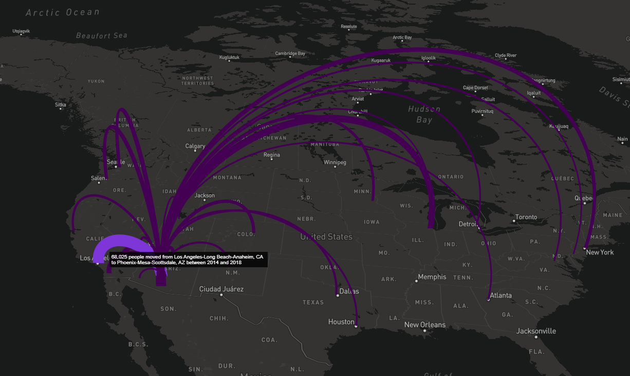
## # ℹ 2 more variables: centroid1 <POINT [°]>, centroid2 <POINT [°]>With the centroids attached to each pair of places, it is straightforward to map the migration flows. Here, we look at the most common origin MSAs for people moving to Phoenix-Mesa-Scottsdale, AZ. To make an interactive map of the flows, we’ll use the excellent mapdeck package. To use mapdeck, you’ll need a Mapbox account and access token.
library(mapdeck)

top_move_in <- phx_flows |>
  filter(!is.na(GEOID2), variable == "MOVEDIN") |>
  slice_max(n = 25, order_by = estimate) |>
  mutate(
    width = estimate / 500,
    tooltip = paste0(
      scales::comma(estimate * 5, 1),
      " people moved from ", str_remove(FULL2_NAME, "Metro Area"),
      " to ", str_remove(FULL1_NAME, "Metro Area"), " between 2014 and 2018"
      )
    )

top_move_in |>
  mapdeck(style = mapdeck_style("dark"), pitch = 45) |>
  add_arc(
    origin = "centroid1",
    destination = "centroid2",
    stroke_width = "width",
    auto_highlight = TRUE,
    highlight_colour = "#8c43facc",
    tooltip = "tooltip"
  )