Getting Started

freestiler is a vector tile engine for R (and Python) that creates PMTiles archives from spatial data. You give it an sf object, a file on disk, or a DuckDB query, and it writes a single .pmtiles file you can serve from anywhere. The engine is written in Rust and runs in-process, so there’s nothing else to install.

The package supports two tile formats: MapLibre Tiles (MLT), a next-generation columnar format that’s the default, and Mapbox Vector Tiles (MVT), the widely-supported protobuf format. See the MapLibre Tiles article for more on the differences.

Installation

Install from r-universe:

install.packages(
  "freestiler",
  repos = c("https://walkerke.r-universe.dev", "https://cloud.r-project.org")
)

The r-universe build includes the Rust DuckDB backend on macOS and Linux, which powers the streaming point pipeline in freestile_query(). You can also install from GitHub with devtools::install_github("walkerke/freestiler").

For Python, see the Python Setup article.

Your first tileset

The main function is freestile(). Let’s tile the North Carolina counties dataset that ships with sf:

library(sf)
library(freestiler)

nc <- st_read(system.file("shape/nc.shp", package = "sf"))

freestile(nc, "nc_counties.pmtiles", layer_name = "counties")

Creating MLT tiles (zoom 0-14) for 100 features across 1 layer...
  Tiling layer 'counties' (zoom 0-14)...
Created nc_counties.pmtiles (65.2 KB)

That’s useful for verifying your installation, but let’s try something more interesting.

A more interesting example

Let’s tile all 242,000 US block groups from the tigris package. This takes about 20 seconds on my machine and produces a tileset you can zoom into from the national level down to individual neighborhoods:

library(tigris)
options(tigris_use_cache = TRUE)

bgs <- block_groups(cb = TRUE)

freestile(
  bgs,
  "us_bgs.pmtiles",
  layer_name = "bgs",
  min_zoom = 4,
  max_zoom = 12
)

Viewing tiles

The quickest way to view a tileset is view_tiles(), which starts a local HTTP server and creates an interactive map in one step:

view_tiles("us_bgs.pmtiles")

It auto-detects the layer name and geometry type from the PMTiles metadata, so it works out of the box for polygon, line, and point data.

For more control over styling and layers, use serve_tiles() to start the server separately and build your map with mapgl. See the Mapping with mapgl article for a full walkthrough of this workflow.

The built-in server handles CORS and HTTP range requests automatically. For tilesets larger than ~1 GB, you’ll get better performance from an external server:

npx http-server /path/to/tiles -p 8082 --cors -c-1

MLT vs MVT

The default tile format is MLT, which tends to produce smaller files for polygon-heavy data. If you need maximum viewer compatibility - particularly for Python viewers or older MapLibre versions - use MVT:

freestile(nc, "nc_mvt.pmtiles", layer_name = "counties", tile_format = "mvt")

Controlling zoom levels

Use min_zoom and max_zoom to set the zoom range for your tileset:

freestile(nc, "nc_z4_10.pmtiles",
  layer_name = "counties",
  min_zoom = 4,
  max_zoom = 10
)

Feature dropping for large datasets

For large datasets, drop_rate provides exponential feature thinning at lower zoom levels. Points are thinned using spatial ordering to maintain even coverage; polygons and lines are thinned by area. The base_zoom parameter controls the zoom level above which all features are kept:

freestile(nc, "nc_dropping.pmtiles",
  layer_name = "counties",
  drop_rate = 2.5,
  base_zoom = 10
)

Direct file input

You can tile spatial files on disk without loading them into R first. This is useful for large GeoParquet files or other formats you’d rather not pull into memory:

# GeoParquet
freestile_file("census_blocks.parquet", "blocks.pmtiles")

# GeoPackage, Shapefile, or other formats via DuckDB
freestile_file("counties.gpkg", "counties.pmtiles", engine = "duckdb")

DuckDB queries

If your data already lives in DuckDB, you can run a SQL query and pipe the results directly into the tiling engine. This lets you filter, join, and transform your data with SQL before tiling:

freestile_query(
  "SELECT * FROM ST_Read('counties.shp') WHERE pop > 50000",
  "large_counties.pmtiles"
)

For very large point datasets, set streaming = "always" to use the streaming pipeline, which avoids loading the full query result into memory:

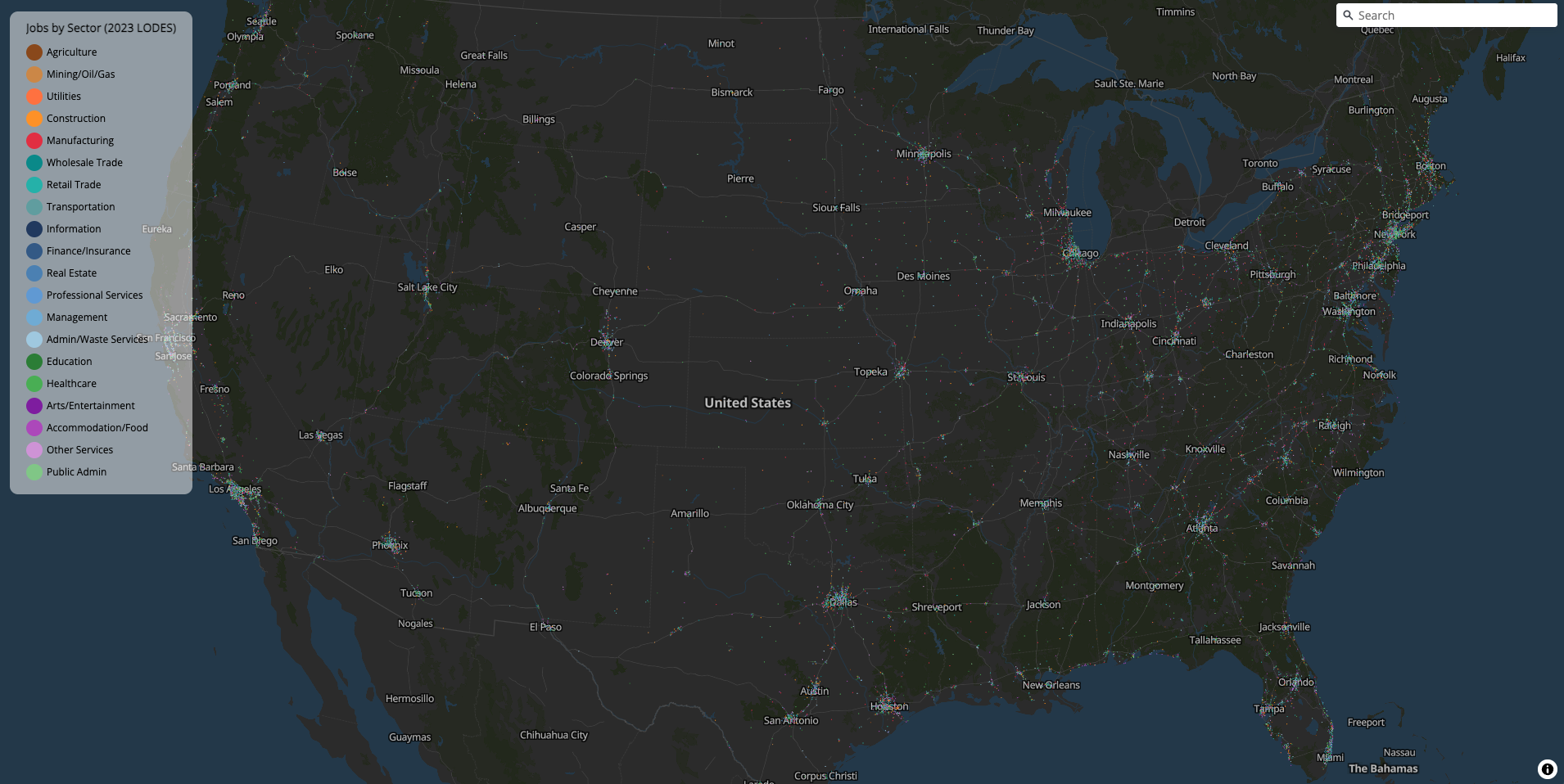
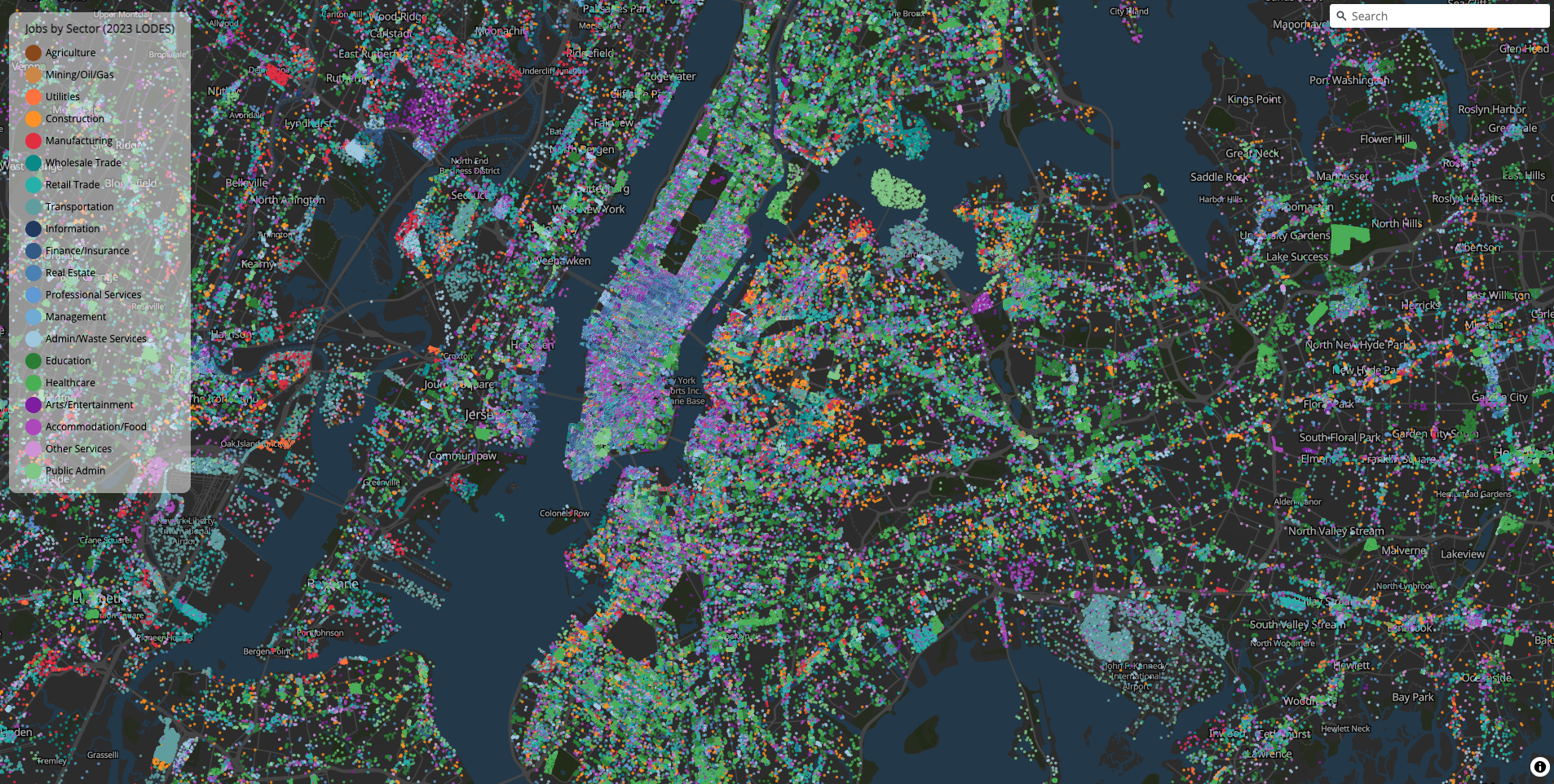
freestile_query(
  query = "SELECT naics, state, ST_Point(lon, lat) AS geometry FROM jobs_dots",
  output = "us_jobs_dots.pmtiles",
  db_path = db_path,
  layer_name = "jobs",
  tile_format = "mvt",
  min_zoom = 4,
  max_zoom = 14,
  base_zoom = 14,
  drop_rate = 2.5,
  source_crs = "EPSG:4326",
  streaming = "always",
  overwrite = TRUE
)

On a recent run, this streamed 146 million US job points from DuckDB into a 2.3 GB PMTiles archive in about 12 minutes.

Multi-layer tilesets

Pass a named list to create multi-layer tilesets. Use freestile_layer() if you want per-layer zoom control:

pts <- st_centroid(nc)

freestile(
  list(
    counties = freestile_layer(nc, min_zoom = 0, max_zoom = 10),
    centroids = freestile_layer(pts, min_zoom = 6, max_zoom = 14)
  ),
  "nc_layers.pmtiles"
)

Point clustering

For point layers, cluster_distance merges nearby points into clusters with a point_count attribute:

freestile(pts, "nc_clustered.pmtiles",
  layer_name = "centroids",
  cluster_distance = 50,
  cluster_maxzoom = 8
)

Feature coalescing

The coalesce parameter merges features with identical attributes within each tile. Lines sharing endpoints are joined, and polygons are grouped into MultiPolygons:

freestile(nc, "nc_coalesced.pmtiles",
  layer_name = "counties",
  coalesce = TRUE
)