geosam provides an R interface to Meta’s Segment Anything Model 3 (SAM3) for detecting objects in satellite imagery and photos. Unlike traditional computer vision approaches, SAM3 lets you describe what you’re looking for in plain text—no training data or model fine-tuning required.
The package is inspired by the Python package segment-geospatial by Qiusheng Wu, and aims to bring similar functionality to R users. geosam offers an R-native API, linking to packages such as terra for spatial workflows and magick for image manipulation. It also includes tools for interactive viewing and extraction with the mapgl R package.
Installation
Getting set up with geosam takes a few steps. First, install from R-Universe:
install.packages("geosam", repos = c("https://walkerke.r-universe.dev", "https://cloud.r-project.org"))
Or, install from source:
pak::pak("walkerke/geosam")
Once installed, load the package then set up a SAM3 Python environment with geosam_install(). By default, if run with no arguments, geosam_install() will use uv for the Python environment.
This creates a dedicated uv environment with PyTorch and HuggingFace transformers.
If you prefer to use venv or conda for Python environment management, you can supply the appropriate argument to geosam_install():
This will set up a Python environment named geosam unless you supply an alternative name to envname.
GPU acceleration
SAM3 runs significantly faster with GPU acceleration. If you have an NVIDIA GPU with CUDA support, or an Apple Silicon Mac, geosam will automatically detect and use it. GPU inference is typically 5-10x faster than CPU, which makes a noticeable difference when processing larger areas or multiple detections.
You can verify your GPU is being used with geosam_status() after installation—look for “MPS (Apple Silicon)” or “CUDA” in the PyTorch status line.
Authentication
geosam uses Meta’s SAM3 model hosted on HuggingFace, which requires authentication and gated model access. You’ll need to complete two steps: accept access terms for the model, and set up your access token.
Requesting SAM3 access
First, visit the SAM3 model page on HuggingFace and click “Request access.” You’ll need a free HuggingFace account and you may be asked to share contact information under the model’s gated access terms. Access is typically granted quickly, but it is still required before geosam can download the weights.
Setting up your access token
Once you have access, you’ll need a User Access Token. From your HuggingFace account, go to Settings > Access Tokens and create a new token. A “read” token is sufficient for geosam since we’re only downloading model weights—and read tokens are safer in case your token is accidentally exposed.
The easiest way to authenticate is to save the token on your machine using the HuggingFace CLI. From your terminal:
This saves your token to ~/.cache/huggingface/token, where geosam will find it automatically.
Alternatively, you can set the token as an environment variable in R. For persistent use across sessions, add it to your .Renviron file:
# Open your .Renviron file
usethis::edit_r_environ()

# Add this line:
# HF_TOKEN=hf_xxxxx
Or set it for a single session:
Imagery API keys
For satellite imagery, geosam supports three providers. Mapbox offers high-quality imagery but requires an API key:
Esri World Imagery works without any API key, making it a good option for getting started. MapTiler is also supported with the MAPTILER_API_KEY environment variable.
Check your setup
Before running your first detection, verify that everything is configured correctly:
── geosam Status ───────────────────────────────────────────────────────────────
ℹ Environment: uv at /Users/kylewalker/.geosam/venvs/geosam
ℹ Path: /Users/kylewalker/.geosam/venvs/geosam/bin/python
✔ PyTorch 2.10.0: MPS (Apple Silicon)
✔ transformers: SAM3 classes available
✔ SAM3 tracker classes: available
✔ HuggingFace token: configured
── SAM3 HuggingFace Access ──
ℹ SAM3 model cache: not found yet
✔ facebook/sam3 access: verified
This will show you the status of your Python environment, whether GPU acceleration is available (MPS on Apple Silicon, CUDA on NVIDIA), whether your HuggingFace token is configured, and whether that token can access facebook/sam3. If everything shows green checkmarks, you’re ready to go.
Troubleshooting conda installations
If you have multiple conda distributions installed (e.g., miniconda, miniforge, anaconda), you may encounter errors like “conda environment ‘geosam’ not found” even when the environment exists. This happens because R’s reticulate package may be looking in a different conda installation than where your environment was created.
To diagnose the issue:
This will scan your system for all conda installations and geosam environments, and provide recommendations. If your geosam environment is in a different conda than reticulate’s default, you can specify which conda to use:
# Use a specific conda installation (e.g., miniforge on Windows)
geosam_install(method = "conda", conda = "C:\\Users\\YourName\\miniforge3\\Scripts\\conda.exe")

# Or on macOS/Linux
geosam_install(method = "conda", conda = "~/miniforge3/bin/conda")
Your first detection
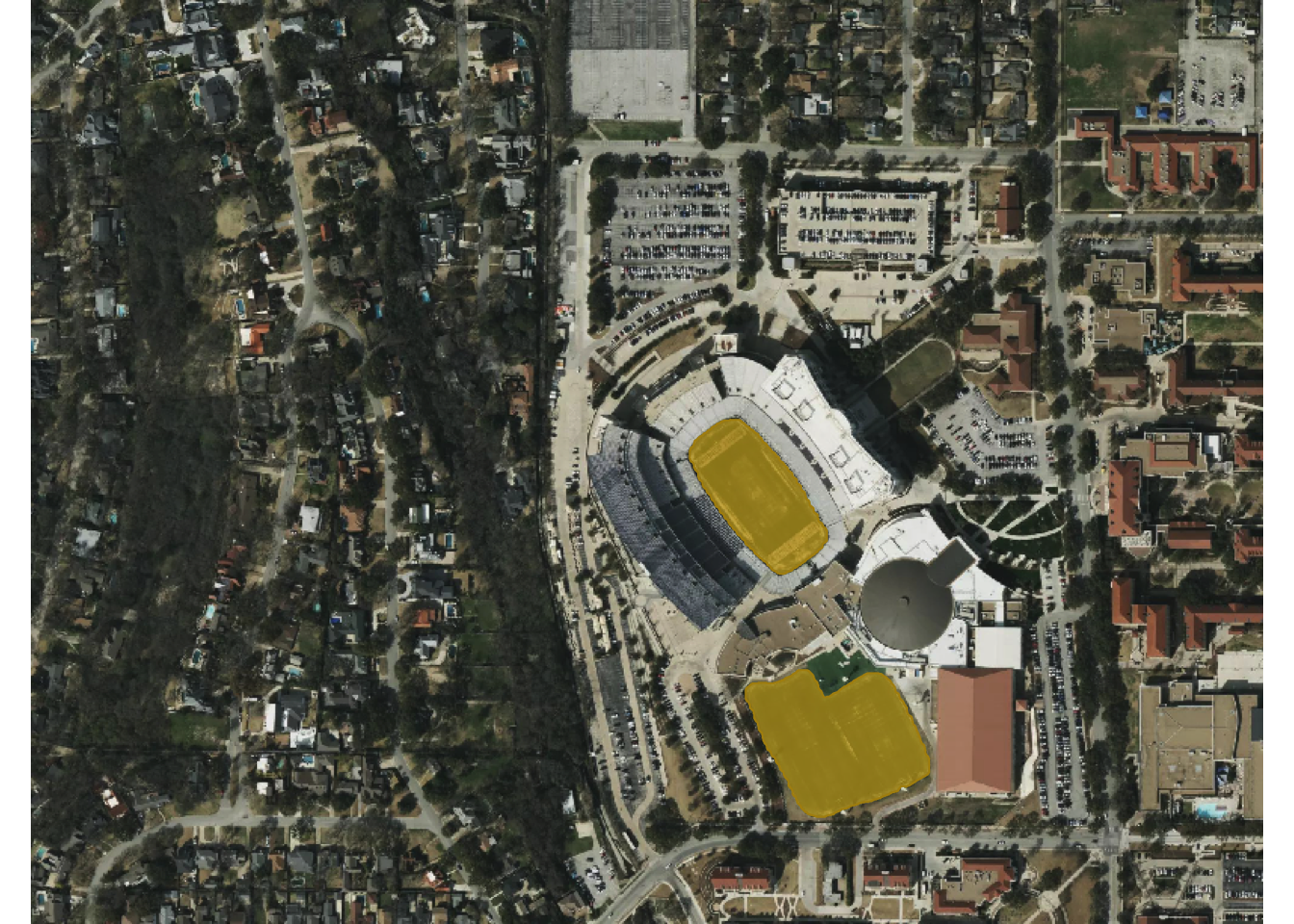
Let’s detect football fields on the TCU campus in Fort Worth. The sam_detect() function is the main workhorse for satellite imagery detection. You provide a bounding box, describe what you’re looking for with a text prompt, and geosam handles the rest—downloading imagery, running SAM3 inference, and returning georeferenced results.
field <- sam_detect(
  bbox = c(-97.372, 32.707, -97.366, 32.712),
  text = "football field",
  source = "mapbox",
  zoom = 17
)
ℹ Mapbox imagery is governed by the Mapbox Terms of Service.
  See: <https://www.mapbox.com/legal/tos/>
ℹ Downloading Mapbox imagery at zoom 17...

ℹ Fetching 12 tiles (4x3)...

✔ Saved imagery to: /var/folders/qm/xbtsglmj2ss91z9fzpz8k6q8ylngb5/T//RtmpuDkU0y/file453853f1b412.tif

ℹ Large image (2048x1536). Processing in 6 chunks...

ℹ Loading SAM3 model...

✔ SAM3 model loaded.

Detecting objects [2/6]  33%

Detecting objects [3/6]  50%

Detecting objects [4/6]  67%

Detecting objects [5/6]  83%

Detecting objects [6/6] 100%

✔ Detected 2 objects across 6 chunks.
The bbox argument takes coordinates in WGS84 (longitude/latitude) as c(xmin, ymin, xmax, ymax). You can also pass an sf object and geosam will extract its bounding box automatically.
The first time you run a detection, SAM3 will download model weights from HuggingFace (about 2.5 GB). This only happens once as subsequent runs use the cached model.
Viewing results
Use sam_view() to explore your detections interactively:
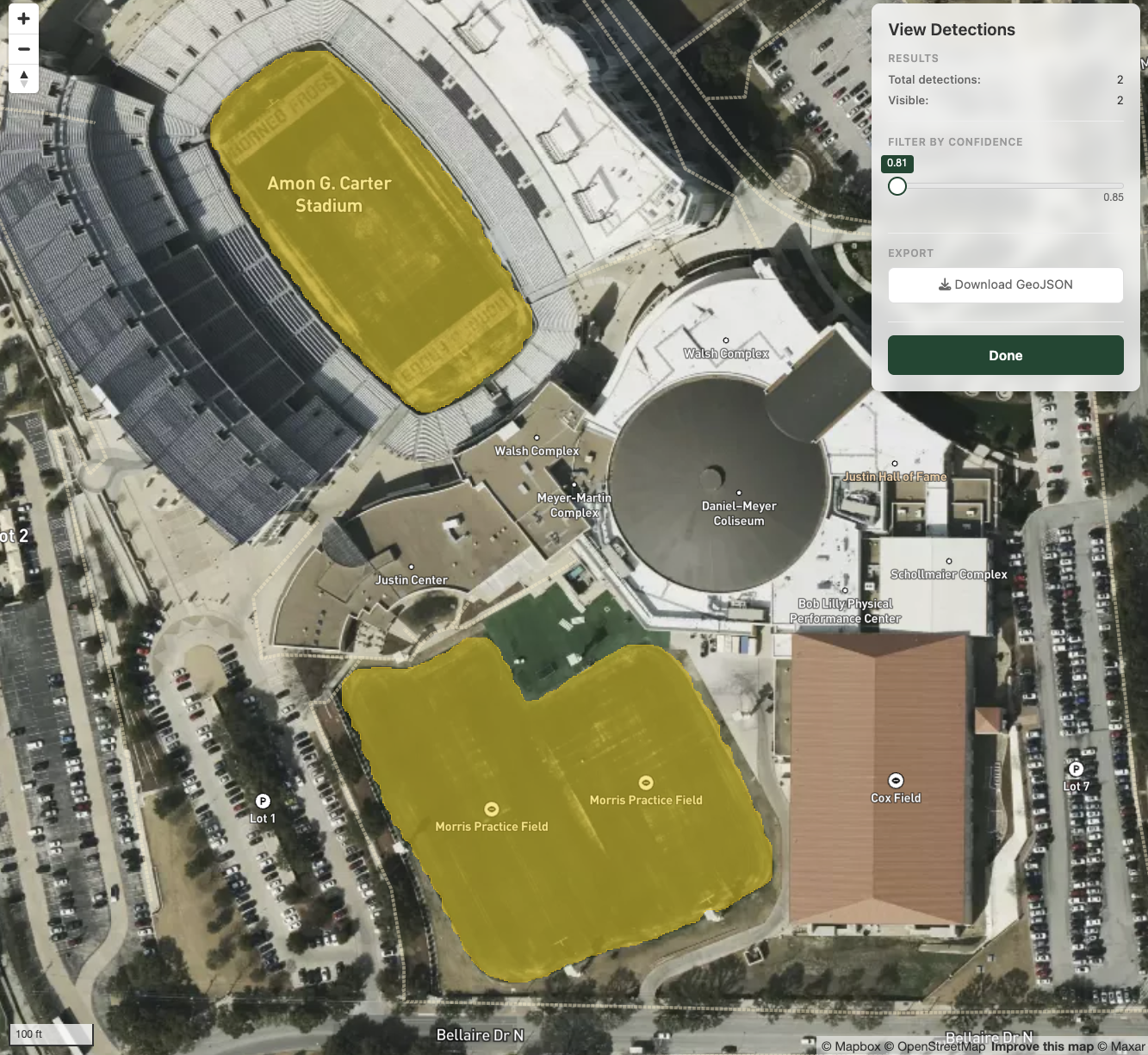
This opens a Shiny application with the satellite imagery as a basemap and your detections overlaid as polygons. You can adjust the confidence threshold with a slider to filter out lower-quality detections, and click on individual polygons to see their confidence scores. Here, we’ve picked up the field inside the football stadium as well as the nearby practice field.
Zoom out a bit for this view - you’ll see a white box representing the extraction area. This is the area that we searched for features matching the text prompt.
When you’re ready to work with the results in R, extract them as an sf object:
Simple feature collection with 2 features and 2 fields
Geometry type: POLYGON
Dimension:     XY
Bounding box:  xmin: -97.3687 ymin: 32.70723 xmax: -97.36657 ymax: 32.71022
Geodetic CRS:  +proj=longlat +datum=WGS84 +no_defs
      score  area_m2                       geometry
1 0.8820943 17306.76 POLYGON ((-97.36768 32.7083...
2 0.8899280 11331.49 POLYGON ((-97.36831 32.7102...
The resulting sf object includes a score column with confidence values (0–1) and an area_m2 column with the area of each detection in square meters. From here, you can filter, analyze, or export your detections using standard sf workflows.