library(geosam)

imagery <- get_imagery(
  bbox = c(-118.41, 34.09, -118.405, 34.095),
  source = "mapbox",
  zoom = 18
)

imagery
[1] "/var/folders/qm/xbtsglmj2ss91z9fzpz8k6q8ylngb5/T//RtmpTwwYUP/file46465bdc5375.tif"With geosam, you can detect objects in satellite imagery using natural language prompts. Describe what you’re looking for, and SAM3 returns georeferenced polygons.
The package hooks SAM3 into R’s geospatial infrastructure, using the terra package for raster processing and mapgl for interactive visualization. Let’s get started!
If you don’t have satellite imagery to use, you can download imagery with geosam from Mapbox, Esri World Imagery, or MapTiler with the get_imagery() function. Let’s grab imagery from Mapbox for a section of Beverly Hills, California:
library(geosam)
imagery <- get_imagery(
bbox = c(-118.41, 34.09, -118.405, 34.095),
source = "mapbox",
zoom = 18
)
imagery[1] "/var/folders/qm/xbtsglmj2ss91z9fzpz8k6q8ylngb5/T//RtmpTwwYUP/file46465bdc5375.tif"The zoom level will control the level of detail in the downloaded imagery, with larger zooms resulting in higher resolution images. The function returns a path to a GeoTIFF file containing the downloaded imagery. We can plot it with the terra package:
You can use this GeoTIFF file as input to the sam_detect() function, or you can simply use sam_detect() to download satellite imagery and run detection in one step. Here we find swimming pools in that section of Beverly Hills:
library(geosam)

pools <- sam_detect(
  bbox = c(-118.41, 34.09, -118.405, 34.095),
  text = "swimming pool",
  source = "mapbox",
  zoom = 18
)

pools
pools is an object of class geosam which represents the extraction result.
To visualize the results of your extraction, use plot():
plot(pools)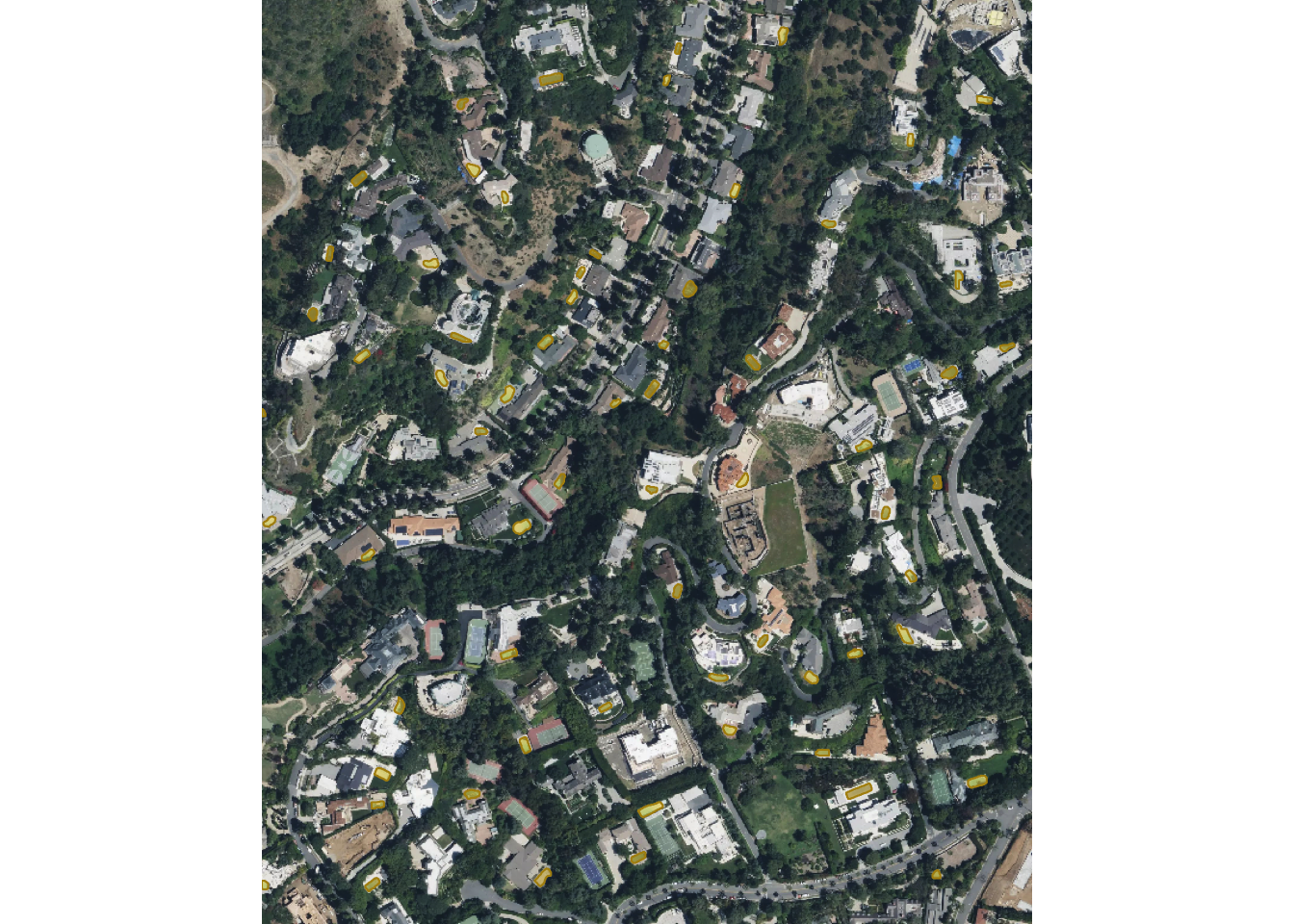
Plotting geosam objects will visualize the extracted polygons on the original imagery. Here, we see the extracted pools visualized in yellow over the Mapbox image.
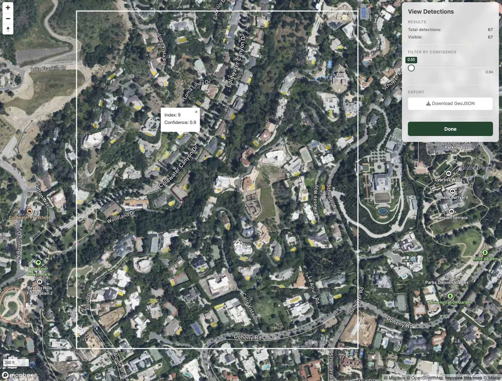
For interactive exploration, use sam_view(). This launches a Shiny app where you can adjust the confidence threshold with a slider, click polygons to see details, and export results as GeoJSON:
sam_view(pools)sam_view() launches a Shiny gadget that gives you an interactive view of your extraction results. The viewer uses the same imagery source (Mapbox, Esri, or MapTiler) as the detection, so results align with the basemap. The white rectangle represents the area SAM3 scanned for extraction results. Click any extracted object to view its index and confidence score (0-1), filter your results by confidence score, and export your result as GeoJSON if you’d like.
Please note the terms of service for the satellite imagery providers. All providers allow for feature extraction from their satellite imagery for non-commercial usage, so you can use this tool for research or analysis purposes. You aren’t allowed to extract data from their imagery and re-sell it. As geosam is MIT-licensed, you alone are responsible for honoring these terms of service in your use of the package.
If you have existing georeferenced satellite or aerial imagery, you can pass the file path directly to use it in sam_detect(). geosam bundles an imagery chip for Mumbai, India from the SpaceNet dataset that you can experiment with. Let’s take a look at it.
# geosam includes a sample WorldView-3 chip from Mumbai (SpaceNet dataset)
mumbai <- system.file("extdata", "mumbai_chip.tif", package = "geosam")

buildings <- sam_detect(
  image = mumbai,
  text = "building"
)

plot(buildings)
sam_detect() found 73 buildings, generally picking out discrete structures but leaving out some of the more densely-packed areas. One reason for this is because sam_detect() defaults to a confidence threshold of 0.5 in its extraction results. If you want to be more generous with the extraction and return all results found by SAM3, you can lower the threshold:
buildings_01 <- sam_detect(
  image = mumbai,
  text = "building",
  threshold = 0.1
)

plot(buildings_01)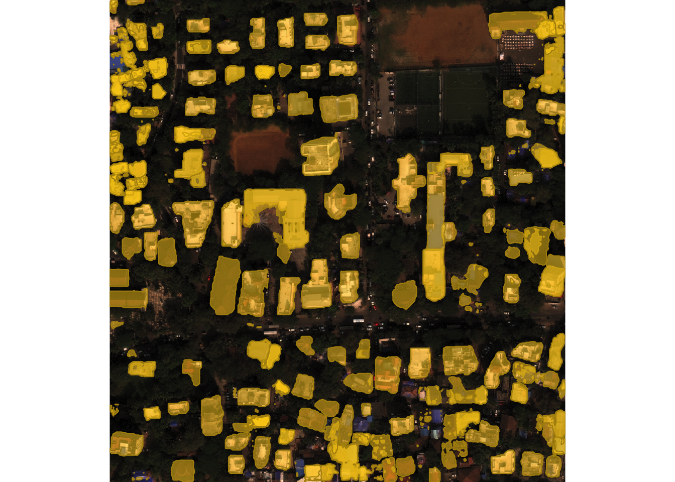
175 objects are now detected, picking up most buildings in the view but also returning some false positives.
Experiment with different types of prompts and see what you get back. For example, we can look for trees in the image:
trees <- sam_detect(image = mumbai, text = "trees", threshold = 0.3)
plot(trees)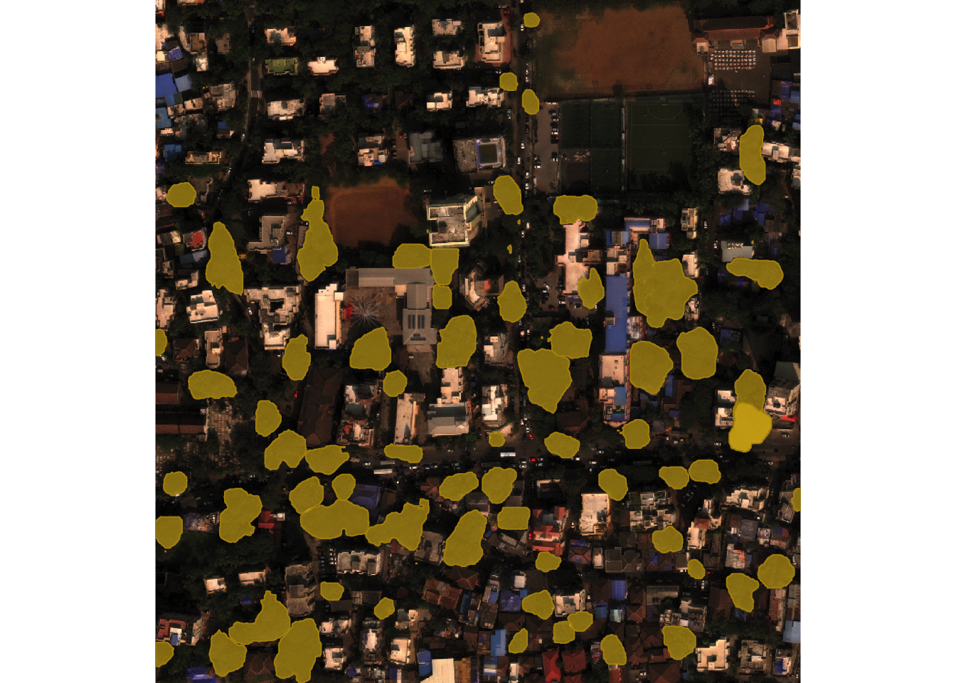
SAM3 also understands color, so you can segment your image by object color as needed.
blue_roofs <- sam_detect(image = mumbai, text = "blue roof", threshold = 0.2)
plot(blue_roofs)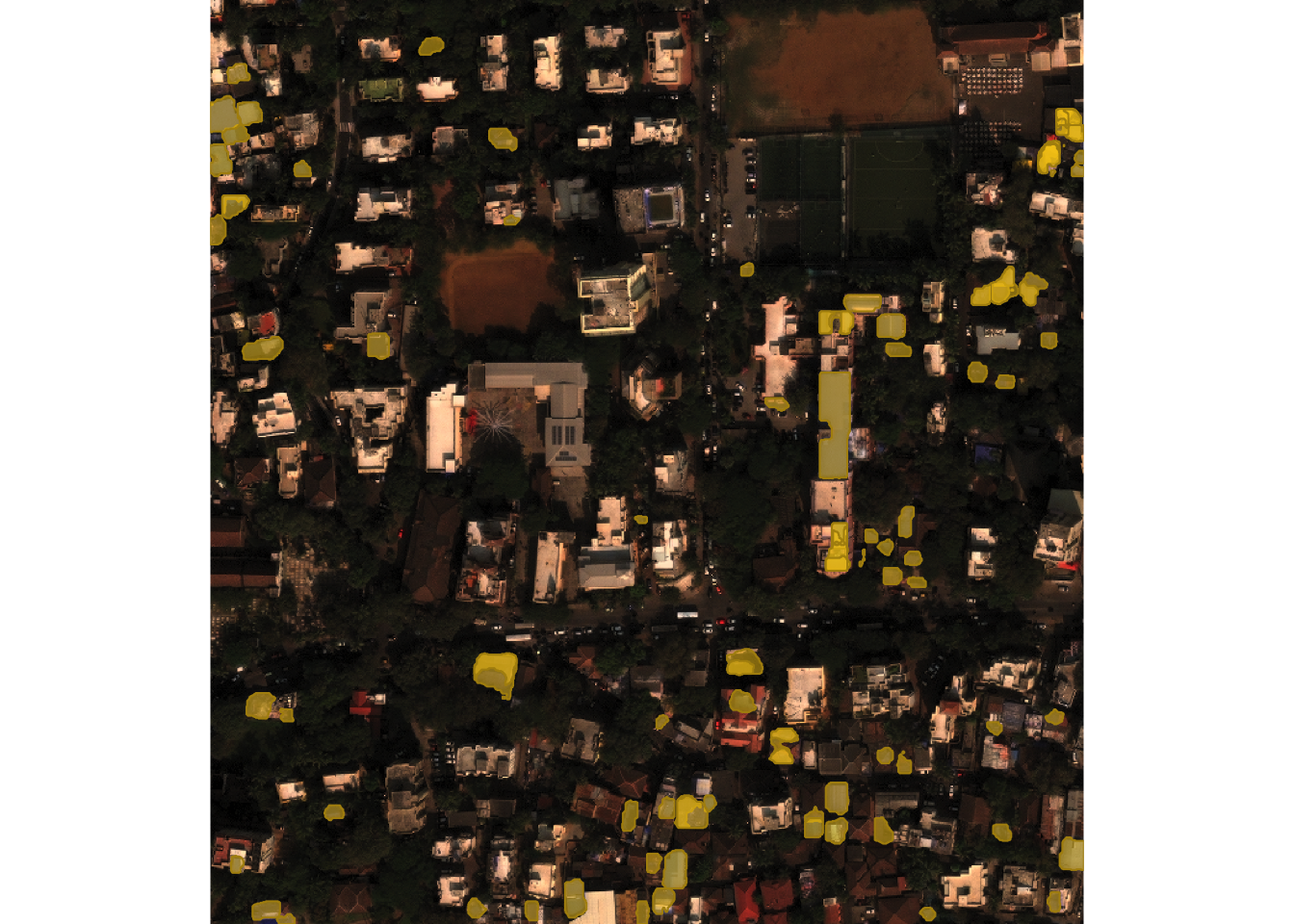
The function sam_as_sf() will convert an object of class geosam to an object of class sf for use in spatial analysis workflows. Let’s convert our original buildings object and see what we get back.
Simple feature collection with 73 features and 3 fields
Geometry type: GEOMETRY
Dimension:     XY
Bounding box:  xmin: 72.82462 ymin: 19.05357 xmax: 72.82827 ymax: 19.05713
Geodetic CRS:  +proj=longlat +datum=WGS84 +no_defs
First 10 features:
       score mask_id                       geometry  area_m2
1  0.5029125       1 POLYGON ((72.82518 19.05373... 315.3316
2  0.7437420       2 POLYGON ((72.82782 19.05632... 246.6490
3  0.6988482       3 POLYGON ((72.82507 19.05541... 315.0516
4  0.7671623       4 POLYGON ((72.82613 19.05438... 282.3758
5  0.5511746       5 POLYGON ((72.82498 19.05641... 184.2481
6  0.7723363       6 POLYGON ((72.82627 19.05674... 174.6477
7  0.6467011       7 POLYGON ((72.82465 19.05568... 248.4039
8  0.6462874       8 POLYGON ((72.82806 19.05647... 249.9719
9  0.7299738       9 POLYGON ((72.82767 19.05611... 171.3253
10 0.6914884      10 POLYGON ((72.82534 19.05692... 210.9247
The result includes polygon geometries, confidence scores, and area in square meters. Use sam_filter() to filter by score or area before extraction:
filtered <- buildings |>
  sam_filter(min_area = 50, min_score = 0.6) |>
  sam_as_sf()

filtered
Simple feature collection with 56 features and 3 fields
Geometry type: GEOMETRY
Dimension: XY
Bounding box: xmin: 72.82462 ymin: 19.05357 xmax: 72.82827 ymax: 19.05712
Geodetic CRS: +proj=longlat +datum=WGS84 +no_defs
First 10 features:
score mask_id geometry area_m2
1 0.7437420 1 POLYGON ((72.82782 19.05632... 246.6490
2 0.6988482 2 POLYGON ((72.82507 19.05541... 315.0516
3 0.7671623 3 POLYGON ((72.82613 19.05438... 282.3758
4 0.7723363 4 POLYGON ((72.82627 19.05674... 174.6477
5 0.6467011 5 POLYGON ((72.82465 19.05568... 248.4039
6 0.6462874 6 POLYGON ((72.82806 19.05647... 249.9719
7 0.7299738 7 POLYGON ((72.82767 19.05611... 171.3253
8 0.6914884 8 POLYGON ((72.82534 19.05692... 210.9247
9 0.7627780 9 POLYGON ((72.82646 19.05582... 492.0996
10 0.6257558 10 POLYGON ((72.82794 19.05379... 315.0546With the sf object in hand, we can use our extracted results downstream in R’s suite of spatial analysis and mapping packages. For example, we can visualize our polygons interactively with the mapgl R package:
library(mapgl)

maplibre_view(buildings_sf)
We notice here that our extractions do not perfectly align with the basemap; this is because our image source and the source of the basemap building footprints are likely slightly different.
This reflects the advantage of using the built-in imagery pipelines with this package as they are pulling directly from the map tiles providers allowing for alignment on your interactive maps.
