Lasso selection and spatial filtering for your Shiny mapping apps

gis

shiny

mapping

Author

Kyle Walker

Published

August 11, 2025

A feature request I commonly get from package users and clients is lasso selection. Lasso selection on a map allows users to interact with a dataset by smoothly drawing a custom shape and getting information back about data within that shape.

Lasso selection can be achieved in mapgl by using the freehand drawing option in the package’s draw control. I’ll show you a couple different ways to achieve the selection portion of lasso-selection: server-side filtering with sf, and client-side filtering with mapgl’s brand-new TurfJS implementation.

As a bonus - I’ll show you at the end of the post how to interact with the ellmer package and get an AI summary of your lasso-selected results.

Getting the data to “lasso”

It’s appropriate to use data from Texas for our “lasso” example, so we’ll use real coffee shop locations in Austin, Texas from Overture Maps. The overtureR package makes this straightforward:

library(overtureR)
library(sf)
library(tidyverse)

# Get Austin city boundary  
austin <- open_curtain("division_area") |>
  filter(subtype == "locality", names$primary == "Austin") |>
  collect()

# Create search area
austin_bbox <- austin |>
  st_geometry() |>
  st_buffer(10000) |>  # 10km buffer for metro area
  st_bbox()

# Get coffee shops
austin_coffee <- open_curtain("place", austin_bbox) |>
  filter(
    str_detect(categories$primary, "coffee") | 
    str_detect(names$primary, "[Cc]offee")
  ) |>
  collect() |>
  filter(!is.na(`names$primary`)) |>
  slice_head(n = 150)

# Save for use in Shiny app
write_rds(austin_coffee, "austin_coffee.rds")

This gives us real coffee shop data that we can load quickly in our Shiny app.

Example: freehand drawing with mapgl

The foundation is mapgl’s draw control with freehand = TRUE, which enables smooth polygon drawing. Try it out below on the interactive map; you’ll draw the polygon by clicking, dragging , then releasing when you are done. I’ve modified the draw control to show a freehand-style polygon button when the freehand option is selected.

library(shiny)
library(readr)
library(mapgl) # pak::pak("walkerke/mapgl") for right now

austin_coffee <- read_rds("austin_coffee.rds")

maplibre(
  style = maptiler_style("streets", variant = "light"),
  bounds = austin_coffee
) |>
  add_circle_layer(
    id = "coffee",
    source = austin_coffee,
    circle_color = "#8B4513",
    circle_radius = 6,
    tooltip = "name"
  ) |>
  add_draw_control(
    position = "top-left",
    freehand = TRUE
  )

This is useful for interactive work (“here’s an area we want to look at”) but to do something with the result, we’ll need to use Shiny to capture the state of our drawings. Let’s step through a couple examples.

Server-side lasso selection with sf

The traditional approach processes drawn polygons server-side using sf:

library(shiny)
library(readr)
library(mapgl)
library(sf)

austin_coffee <- read_rds("austin_coffee.rds")

ui <- fluidPage(
  maplibreOutput("map", height = "500px"),
  h4("Selected Coffee Shops:"),
  textOutput("results")
)

server <- function(input, output, session) {
  output$map <- renderMaplibre({
    maplibre(
      style = maptiler_style("streets", variant = "light"),
      bounds = austin_coffee
    ) |>
      add_circle_layer(
        id = "coffee",
        source = austin_coffee,
        circle_color = "#8B4513",
        circle_radius = 6,
        tooltip = "name"
      ) |>
      add_draw_control(
        position = "top-left",
        freehand = TRUE
      )
  })

  observeEvent(input$map_drawn_features, {
    drawn <- input$map_drawn_features
    
    if (!is.null(drawn)) {
      # Convert to sf and perform spatial filter in R
      drawn_sf <- get_drawn_features(maplibre_proxy("map"))
      selected <- austin_coffee |>
        st_filter(drawn_sf)
      
      # Update results
      output$results <- renderText({
        paste("Selected", nrow(selected), "coffee shops")
      })
    } else {
      output$results <- renderText("")
    }
  })
}

shinyApp(ui, server)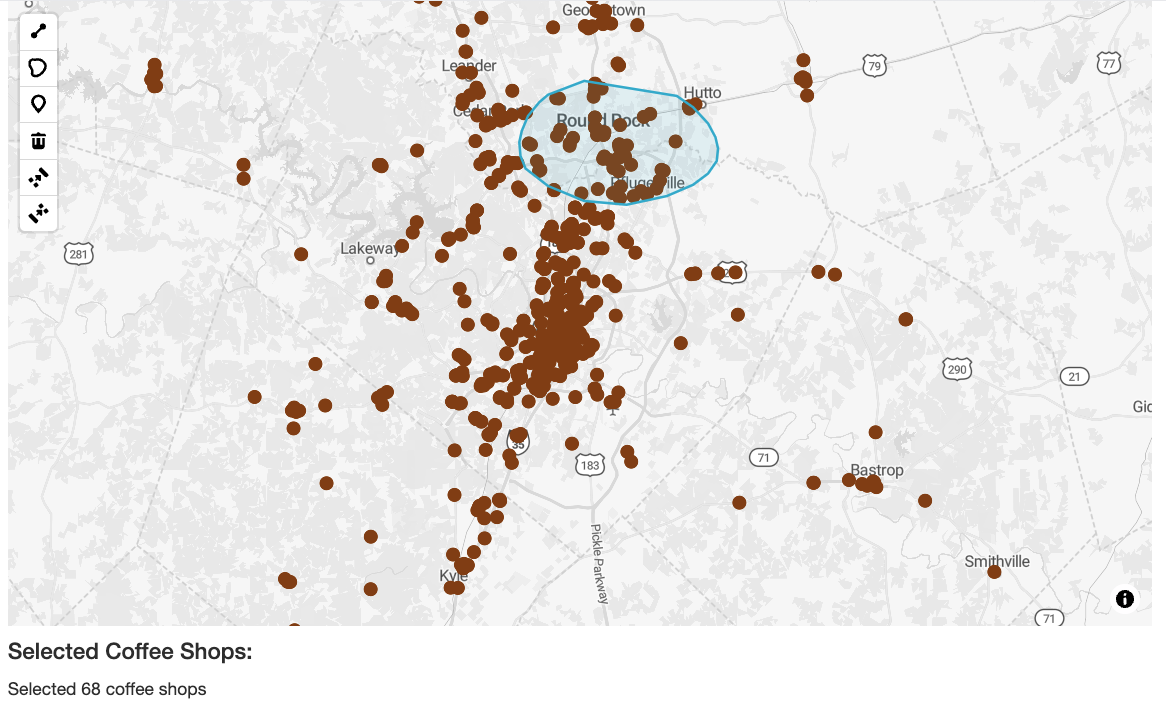

Some notes on how we get this done:

The input$map_drawn_features input (which assumes your map’s ID is "map" in your Shiny app) dynamically updates as you draw on the map. We can observe for its existence, and do lasso selection if the drawing exists. (A caveat - we are assuming here that you’ve drawn a lasso polygon, not points or lines).
get_drawn_features() returns the current drawn features as an sf object to Shiny’s R session, allowing you to use it downstream with sf functions.
In turn, we filter our coffee shops with st_filter(), and print out the number of shops we’ve found.

Client-side lasso selection with `turf_filter()`

The traditional server-side approach typically works quite well. However, as the complexity of your app scales, you may encounter some performance issues with server-side spatial operations, as the lasso selection requires a round-trip between R and JavaScript via Shiny to get its work done.

An alternative approach uses mapgl’s brand-new TurfJS integration. I’ve added a variety of commonly-used TurfJS functions to mapgl to assist with in-browser, client-side spatial analysis. A custom function, turf_filter(), is one of my favorites. It allows you to to client-side data filtering akin to st_filter(), invoking TurfJS’s boolean overlay functions internally.

Let’s make the app a bit more complex, displaying selected points on the map as we filter them.

library(shiny)
library(mapgl)

austin_coffee <- read_rds("austin_coffee.rds")

ui <- fluidPage(
  maplibreOutput("map", height = "500px"),
  h4("Selected Coffee Shops:"),
  textOutput("results")
)

server <- function(input, output, session) {
  output$map <- renderMaplibre({
    maplibre(
      style = maptiler_style("streets", variant = "light"),
      bounds = austin_coffee
    ) |>
      add_circle_layer(
        id = "coffee",
        source = austin_coffee,
        circle_color = "#8B4513",
        circle_stroke_color = "white",
        circle_radius = 6,
        tooltip = "name"
      ) |>
      add_draw_control(
        position = "top-left",
        freehand = TRUE
      )
  })
  
  observeEvent(input$map_drawn_features, {
    # Quick pause to avoid race conditions
    Sys.sleep(0.2)
    maplibre_proxy("map") |> 
      turf_filter(
        layer_id = "coffee",
        filter_layer_id = "gl-draw-polygon-fill.cold",
        predicate = "within",
        source_id = "selected",
        input_id = "results"
      ) 
  })
  
  observeEvent(input$map_turf_results, {
    maplibre_proxy("map") |> 
      clear_layer("highlights") 
    
    if (!is.null(input$map_drawn_features)) {
      maplibre_proxy("map") |> 
        add_circle_layer(
        id = "highlights",
        source = "selected",
        circle_color = "red",
        circle_radius = 10,
        circle_stroke_color = "white",
        circle_stroke_width = 2
      )
    }
  })

  observeEvent(input$map_turf_results, {
    result <- input$map_turf_results
    count <- length(result$result$features)
    output$results <- renderText({
      paste("Selected", count, "coffee shops")
    })
  })
}

shinyApp(ui, server)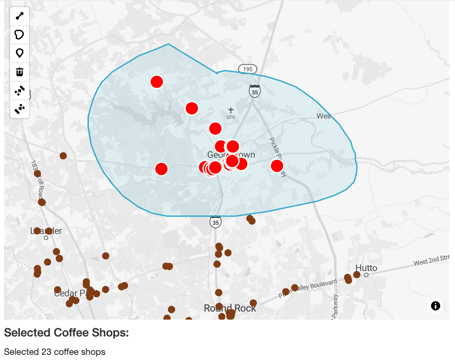

With respect to the implementation here:

Results come back from the TurfJS filter operation instantly, and are stored in input$map_turf_results. Note that "map" is the Map ID, and "results" is the Turf ID we specified in turf_filter().
Within turf_filter(), we use the name the draw control gives the drawn polygon; filter_layer_id = "gl-draw-polygon-fill.cold" will work.
Because we are doing client-side work here, we need to pay close attention to race conditions. R users don’t typically think about race conditions, as operations tend to happen sequentially. In web programming, however, this can be a big deal - as you may be trying to do something that depends on a process that hasn’t finished yet. This shows up in our app where you see the Sys.sleep(0.2) call; I’m pausing for 0.2 seconds to allow the drawn polygon to be registered as a source on the map before we try to filter data with it.

Streaming AI insights about selected features

Finally, let’s add AI analysis of the selected coffee shops using the ellmer and shinychat packages, with an approach borrowed from my last blog post! Try the app out - it’s a fun example of how you can integrate interactive responses with generative AI with the lasso selection approach outlined in this post.

Code

library(shiny)
library(mapgl)
library(ellmer)
library(shinychat)
library(bslib)

# Load coffee shop data
austin_coffee <- readRDS("austin_coffee.rds")

# Initialize Claude Sonnet
llm_chat <- NULL
if (nchar(Sys.getenv("ANTHROPIC_API_KEY")) > 0) {
  llm_chat <- chat_anthropic(
    model = "claude-sonnet-4-20250514",
    system_prompt = "You are a local business analyst. Provide brief, interesting insights about coffee shop locations and patterns. Keep responses concise and engaging."
  )
}

ui <- page_fluid(
  tags$head(
    tags$style(HTML(
      "
      body, .container-fluid {
        padding: 0;
        margin: 0;
      }
      .floating-panel {
        position: absolute;
        top: 10px;
        left: 10px;
        z-index: 1000;
        background: rgba(255, 255, 255, 0.95);
        padding: 15px;
        border-radius: 8px;
        box-shadow: 0 2px 10px rgba(0,0,0,0.1);
        width: 300px;
        max-height: 80vh;
        overflow-y: auto;
        backdrop-filter: blur(5px);
      }
      #map {
        position: absolute;
        top: 0;
        bottom: 0;
        width: 100%;
      }
    "
    ))
  ),

  maplibreOutput("map", height = "100vh"),

  absolutePanel(
    class = "floating-panel",
    h5("Austin Coffee Lasso Selection"),
    p(
      "Draw a polygon to select coffee shops, then ask AI about them.",
      style = "font-size: 14px;"
    ),

    textOutput("count"),
    textOutput("sample_names"),

    conditionalPanel(
      condition = "output.ai_enabled && output.has_selection",
      br(),
      actionButton(
        "analyze",
        "Ask AI about selection",
        class = "btn-primary btn-sm",
        width = "100%"
      ),
      br(),
      br(),
      output_markdown_stream("ai_response")
    )
  )
)

server <- function(input, output, session) {
  # Track current selection
  current_selection <- reactiveVal(list())

  output$map <- renderMaplibre({
    maplibre(
      style = maptiler_style("streets", variant = "light"),
      bounds = austin_coffee
    ) |>
      add_circle_layer(
        id = "coffee",
        source = austin_coffee,
        circle_color = "#8B4513",
        circle_radius = 6,
        circle_stroke_color = "white",
        circle_stroke_width = 1,
        tooltip = "name"
      ) |>
      add_draw_control(
        position = "top-right",
        freehand = TRUE
      )
  })

  # Track AI availability and selection status
  output$ai_enabled <- reactive({
    !is.null(llm_chat)
  })
  output$has_selection <- reactive({
    length(current_selection()) > 0
  })
  outputOptions(output, "ai_enabled", suspendWhenHidden = FALSE)
  outputOptions(output, "has_selection", suspendWhenHidden = FALSE)

  # Handle drawing events
  observeEvent(input$map_drawn_features, {
    drawn <- input$map_drawn_features

    if (!is.null(drawn)) {
      maplibre_proxy("map") |>
        clear_layer("highlights")

      Sys.sleep(0.2)

      maplibre_proxy("map") |>
        turf_filter(
          layer_id = "coffee",
          filter_layer_id = "gl-draw-polygon-fill.cold",
          predicate = "within",
          source_id = "selected",
          input_id = "results"
        )
    } else {
      current_selection(list())
      output$count <- renderText("")
      output$sample_names <- renderText("")

      maplibre_proxy("map") |>
        clear_layer("highlights")
    }
  })

  # Handle filter results
  observeEvent(input$map_turf_results, {
    result <- input$map_turf_results

    maplibre_proxy("map") |>
      clear_layer("highlights") |>
      add_circle_layer(
        id = "highlights",
        source = "selected",
        circle_color = "red",
        circle_radius = 10,
        circle_stroke_color = "white",
        circle_stroke_width = 2
      )

    if (!is.null(result$result$features)) {
      features <- result$result$features
      current_selection(features)

      shop_names <- sapply(features, function(f) f$properties$name)

      output$count <- renderText({
        paste("Selected", length(features), "coffee shops")
      })

      output$sample_names <- renderText({
        if (length(shop_names) > 0) {
          sample_size <- min(3, length(shop_names))
          paste0(
            "Sample: ",
            paste(head(shop_names, sample_size), collapse = ", ")
          )
        }
      })
    }
  })

  # Handle AI analysis button click
  observeEvent(input$analyze, {
    features <- current_selection()

    if (length(features) > 0 && !is.null(llm_chat)) {
      shop_names <- sapply(features, function(f) f$properties$name)

      # Create detailed prompt
      prompt <- paste0(
        "I've selected ",
        length(features),
        " coffee shops in Austin, Texas: ",
        paste(head(shop_names, 8), collapse = ", "),
        if (length(features) > 8)
          paste0(" and ", length(features) - 8, " others"),
        ". What insights can you provide about this area or these businesses? Are there any interesting patterns?"
      )

      # Stream the AI response
      stream <- llm_chat$stream_async(prompt)

      markdown_stream(
        id = "ai_response",
        content_stream = stream,
        operation = "replace"
      )
    }
  })
}

shinyApp(ui, server)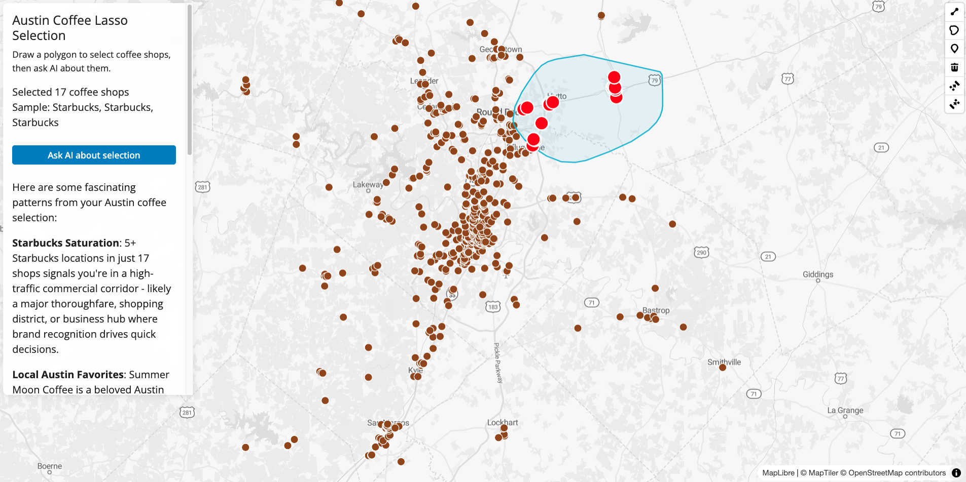

Lasso selection can be a great tool to enhance interactivity on your Shiny mapping apps for your users. With respect to choosing between server-side and client-side filtering, I’d recommend experimenting with both for your use-cases. I tend to prefer client-side interactive filtering for performance reasons, as server-side filtering that appears fast on your local computer may slow down significantly when the app is deployed. That said, using the power of R to do filtering may be helpful when working on large amounts of data that TurfJS / the browser may struggle to handle.

Let me know how you are using these tools! If you want to learn more about new features in mapgl, check out the workshop series I gave in July that covers a ton of useful examples for modernizing your web mapping and app development workflows. I’m also available for custom workshops or consulting to help you integrate these tools into your platforms; feel free to reach out to kyle@walker-data.com.

Getting the data to “lasso”

Example: freehand drawing with mapgl

Server-side lasso selection with sf

Client-side lasso selection with turf_filter()

Streaming AI insights about selected features

Client-side lasso selection with `turf_filter()`