Client-side geospatial analysis with turf.js • mapgl

Why client-side geospatial analysis?

mapgl integrates turf.js v7.2.0 to bring powerful geospatial analysis directly to the browser. This means you can perform spatial operations like buffering, filtering, and overlay analysis without any server round-trips - making your Shiny applications much more responsive and reducing computational load on your server.

This is particularly valuable for deployed applications where you want users to interact with spatial data in real-time without waiting for server processing. Think interactive filtering, drawing tools that immediately show results, or exploratory analysis that responds instantly to user input.

Turf functions in mapgl support three input methods: existing map layer or source references (layer_id), sf objects (data), or raw coordinates when available - giving you flexibility in how you structure your spatial workflows.

Buffering geometries

The turf_buffer() function creates buffer zones around your features. This is useful for proximity analysis, creating catchment areas, or adding visual emphasis around points of interest.

library(mapgl)
library(sf)
library(tigris)
options(tigris_use_cache = TRUE)

# Create a point for Texas Christian University
tcu <- st_sf(
  name = "TCU",
  geometry = st_sfc(st_point(c(-97.364, 32.708)), crs = 4326)
)

# Create a map with TCU and a 2-mile buffer
maplibre(style = carto_style("positron"), 
         center = c(-97.364, 32.708), 
         zoom = 11) |>
  # TCU location
  add_circle_layer(
    id = "tcu",
    source = tcu,
    circle_color = "purple",
    circle_radius = 8,
    circle_stroke_color = "white",
    circle_stroke_width = 2
  ) |>
  # Create 2-mile buffer around TCU
  turf_buffer(
    layer_id = "tcu",
    radius = 2,
    units = "miles",
    source_id = "tcu_buffer"
  ) |>
  # Style the buffer
  add_fill_layer(
    id = "buffer_display",
    source = "tcu_buffer", 
    fill_color = "purple",
    fill_opacity = 0.2,
    fill_outline_color = "purple"
  )

Spatial filtering with predicates

One of the most powerful features is turf_filter(), which lets you filter features based on their spatial relationships. This supports five spatial predicates:

intersects: Features that overlap or touch
within: Features completely inside others
contains: Features that completely contain others
crosses: Features that cross boundaries
disjoint: Features that don’t touch at all

# Find Census tracts that intersect with TCU's 2-mile buffer
tarrant_tracts <- tracts("TX", "Tarrant", cb = TRUE)

maplibre(style = carto_style("positron")) |>
  fit_bounds(tarrant_tracts) |>
  # All Census tracts
  add_fill_layer(
    id = "all_tracts",
    source = tarrant_tracts,
    fill_color = "lightgray",
    fill_opacity = 0.5,
    fill_outline_color = "white"
  ) |>
  # TCU buffer as filter geometry
  turf_buffer(
    data = tcu,
    radius = 2,
    units = "miles",
    source_id = "tcu_buffer_filter"
  ) |> 
  # Find tracts that intersect with the buffer
  turf_filter(
    layer_id = "all_tracts",
    filter_layer_id = "tcu_buffer_filter",
    predicate = "intersects",
    source_id = "intersecting_tracts"
  ) |>
  # Highlight the results
  add_fill_layer(
    id = "intersects_result",
    source = "intersecting_tracts",
    fill_color = "red",
    fill_opacity = 0.8
  ) |>
  # Show TCU location
  add_circle_layer(
    id = "tcu_location",
    source = tcu,
    circle_color = "purple",
    circle_radius = 10,
    circle_stroke_color = "white",
    circle_stroke_width = 3
  ) |> 
  add_fill_layer(
    id = "buffer_display",
    source = "tcu_buffer_filter",
    fill_color = "purple",
    fill_opacity = 0.2
  )

Note how we can chain together turf operations; the layer_id argument supports either source or layer IDs in your map, so you don’t necessarily need to visualize your sources before using them for spatial analysis.

Interactive spatial filtering in Shiny

The real power of client-side spatial analysis shines in Shiny applications. Here’s a simple app that lets users draw polygons and instantly filter counties:

library(shiny)
library(mapgl)
library(sf)
library(tigris)

tarrant_tracts <- tracts(state = "TX", county = "Tarrant", cb = TRUE)

ui <- fluidPage(
  maplibreOutput("map", height = "100vh"),
  
  absolutePanel(
    top = 10, left = 10,
    selectInput("predicate", "Filter Type:",
                choices = c("Intersects" = "intersects",
                            "Within" = "within", 
                            "Contains" = "contains",
                            "Disjoint" = "disjoint"),
                selected = "intersects"),
    
    verbatimTextOutput("results")
  )
)

server <- function(input, output, session) {
  output$map <- renderMaplibre({
    maplibre(style = carto_style("positron")) |>
      fit_bounds(tarrant_tracts) |>
      add_fill_layer(
        id = "tracts",
        source = tarrant_tracts,
        fill_color = "lightblue",
        fill_opacity = 0.5,
        fill_outline_color = "white"
      ) |>
      add_draw_control(position = "top-right")
  })
  
  # Real-time filtering when user draws
  observeEvent(input$map_drawn_features, {
    if (!is.null(input$map_drawn_features)) {
      # Debounce slightly to allow the source to load
      Sys.sleep(0.2)
      maplibre_proxy("map") |>
        turf_filter(
          layer_id = "tracts",
          filter_layer_id = "gl-draw-polygon-fill.cold",
          predicate = input$predicate,
          source_id = "filtered_tracts",
          input_id = "filter_results"
        ) |>
        add_fill_layer(
          id = "filtered",
          source = "filtered_tracts", 
          fill_color = "red",
          fill_opacity = 0.8
        )
    }
  })
  
  output$results <- renderText({
    if (!is.null(input$map_turf_filter_results)) {
      paste("Found", length(input$map_turf_filter_results$result$features), "Census tracts")
    }
  })
}

shinyApp(ui, server)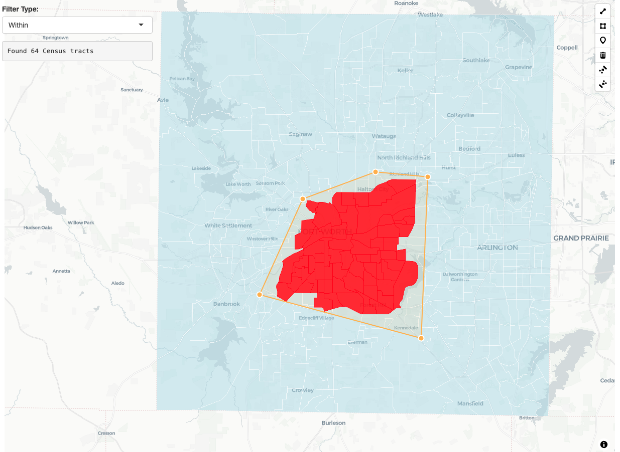

Geometric operations

mapgl includes several geometric analysis functions for more advanced spatial workflows. Let’s create centroids for some Fort Worth area Census tracts and analyze their spatial patterns:

# Get a subset of tracts
fort_worth_tracts <- tarrant_tracts[1:10, ]  # First 10 tracts for demo

maplibre(style = carto_style("positron")) |>
  fit_bounds(fort_worth_tracts) |>
  # Show the tract boundaries
  add_fill_layer(
    id = "tracts",
    source = fort_worth_tracts,
    fill_color = "lightgray",
    fill_opacity = 0.3,
    fill_outline_color = "white"
  ) |>
  # Calculate geometric centroids
  turf_centroid(
    layer_id = "tracts",
    source_id = "centroids"
  ) |>
  # Calculate centers of mass (alternative centroid method)
  turf_center_of_mass(
    layer_id = "tracts", 
    source_id = "mass_centers"
  ) |>
  # Create convex hull around centroids
  turf_convex_hull(
    layer_id = "centroids",
    source_id = "hull"
  ) |>
  # Create Voronoi polygons from centroids
  turf_voronoi(
    layer_id = "centroids", 
    source_id = "voronoi"
  ) |>
  # Style the results
  add_fill_layer(
    id = "hull_display",
    source = "hull",
    fill_color = "blue",
    fill_opacity = 0.2
  ) |>
  add_line_layer(
    id = "voronoi_lines",
    source = "voronoi",
    line_color = "purple",
    line_width = 1
  ) |>
  add_circle_layer(
    id = "centroids_display",
    source = "centroids",
    circle_color = "red",
    circle_radius = 6
  ) |>
  add_circle_layer(
    id = "mass_centers_display", 
    source = "mass_centers",
    circle_color = "orange",
    circle_radius = 4
  )

Note the difference between turf_centroid() (geometric center) and turf_center_of_mass() (area-weighted center) - they may differ for irregular polygons.

Overlay analysis

For more complex spatial analysis, you can combine multiple turf operations. The turf_intersect() function returns the actual intersection geometry - the overlapping area between features:

# Create two overlapping buffer zones around different Fort Worth locations
downtown_fw <- st_sf(geometry = st_sfc(st_point(c(-97.3313, 32.7548)), crs = 4326))  # Downtown
cultural_district <- st_sf(geometry = st_sfc(st_point(c(-97.3632, 32.7494)), crs = 4326))  # Cultural District

maplibre(style = carto_style("positron"), 
         center = c(-97.3313, 32.7548), zoom = 12) |>
  # Create overlapping buffers
  turf_buffer(data = downtown_fw, radius = 1.5, units = "miles", source_id = "downtown_buffer") |>
  turf_buffer(data = cultural_district, radius = 1.5, units = "miles", source_id = "cultural_buffer") |>
  # Show original buffer areas
  add_fill_layer(id = "downtown", source = "downtown_buffer", fill_color = "red", fill_opacity = 0.3) |>
  add_fill_layer(id = "cultural", source = "cultural_buffer", fill_color = "blue", fill_opacity = 0.3) |>
  # Calculate the intersection - returns the overlapping geometry
  turf_intersect(
    layer_id = "downtown_buffer",
    layer_id_2 = "cultural_buffer", 
    source_id = "intersection_result"
  ) |>
  # Show the intersection area
  add_fill_layer(
    id = "intersection",
    source = "intersection_result",
    fill_color = "green",
    fill_opacity = 0.8
  )

We get a buffer “Venn diagram” that shows us areas near to each of the points of interest.

Available functions

mapgl currently supports these turf.js operations:

turf_buffer(): Create buffers around features
turf_filter(): Filter features by spatial predicates
turf_union(): Merge overlapping polygons
turf_intersect(): Return intersection geometry between features
turf_difference(): Subtract one geometry from another
turf_convex_hull(): Create convex boundary around points
turf_concave_hull(): Create fitted boundary around points
turf_voronoi(): Generate Voronoi polygons from points
turf_centroid(): Find centroids as mean of all object vertices
turf_center_of_mass(): Alternative centroid method (will be more similar to sf::st_centroid())
turf_distance(): Calculate distances (Shiny only)
turf_area(): Calculate areas (Shiny only)

Each function supports flexible input methods and integrates seamlessly with mapgl’s layer system, giving you powerful spatial analysis capabilities right in the browser.