Working with Decennial Census Data in R

2025 SSDAN Webinar Series

Kyle Walker

2025-02-12

About me

Professor of Geography at TCU
Spatial data science researcher and consultant
Package developer: tidycensus, tigris, mapgl, mapboxapi, crsuggest, idbr (R), pygris (Python)
Book: Analyzing US Census Data: Methods, Maps and Models in R

SSDAN webinar series

Wednesday, February 5: Analyzing Data from the 2023 American Community Survey in R
Today: Working with Decennial Census Data in R
Wednesday, February 26: Mapping and Spatial Analysis with US Census Data in R

Today’s agenda

Hour 1: Getting started with 2020 Decennial US Census data in R
Hour 2: Analysis workflows with 2020 Census data
Hour 3: The detailed DHC data files and time-series analysis

Getting started with 2020 Decennial US Census data in R

R and RStudio

R: programming language and software environment for data analysis (and wherever else your imagination can take you!)
RStudio: integrated development environment (IDE) for R developed by Posit
Posit Cloud: run RStudio with today’s workshop pre-configured at https://posit.cloud/content/9689451

What is the decennial US Census?

Complete count of the US population mandated by Article 1, Sections 2 and 9 in the US Constitution
Directed by the US Census Bureau (US Department of Commerce); conducted every 10 years since 1790
Used for proportional representation / congressional redistricting
Limited set of questions asked about race, ethnicity, age, sex, and housing tenure

The 2020 US Census: available datasets

Available datasets from the 2020 US Census include:

The PL 94-171 Redistricting Data
The Demographic and Housing Characteristics (DHC) file
The Demographic Profile (for pre-tabulated variables)
Tabulations for the 118th Congress & for Island Areas
The Detailed DHC-A file (with very detailed racial & ethnic categories)
The Detailed DHC-B file (with housing characteristics for those detailed categories)

How to get decennial Census data

data.census.gov is the main, revamped interactive data portal for browsing and downloading Census datasets
The US Census Application Programming Interface (API) allows developers to access Census data resources programmatically

tidycensus

R interface to the Decennial Census, American Community Survey, Population Estimates Program, and Public Use Microdata Series APIs
First released in 2017; over 600,000 downloads from the Posit CRAN mirror

tidycensus: key features

Wrangles Census data internally to return tidyverse-ready format (or traditional wide format if requested);
Automatically downloads and merges Census geometries to data for mapping;
Includes a variety of analytic tools to support common Census workflows;
States and counties can be requested by name (no more looking up FIPS codes!)

Getting started with tidycensus

To get started, install the packages you’ll need for today’s workshop
If you are using the Posit Cloud environment, these packages are already installed for you

install.packages(c("tidycensus", "tidyverse", "mapview"))

Optional: your Census API key

tidycensus (and the Census API) can be used without an API key, but you will be limited to 500 queries per day
Power users: visit https://api.census.gov/data/key_signup.html to request a key, then activate the key from the link in your email.
Once activated, use the census_api_key() function to set your key as an environment variable

library(tidycensus)

census_api_key("YOUR KEY GOES HERE", install = TRUE)

Getting started with Census data in tidycensus

2020 Census data in tidycensus

The get_decennial() function is used to acquire data from the decennial US Census
The two required arguments are geography and variables for the functions to work; for 2020 Census data, use year = 2020.

pop20 <- get_decennial(
  geography = "state",
  variables = "P1_001N",
  year = 2020
)

Decennial Census data are returned with four columns: GEOID, NAME, variable, and value

pop20

# A tibble: 52 × 4
   GEOID NAME                 variable    value
   <chr> <chr>                <chr>       <dbl>
 1 42    Pennsylvania         P1_001N  13002700
 2 06    California           P1_001N  39538223
 3 54    West Virginia        P1_001N   1793716
 4 49    Utah                 P1_001N   3271616
 5 36    New York             P1_001N  20201249
 6 11    District of Columbia P1_001N    689545
 7 02    Alaska               P1_001N    733391
 8 12    Florida              P1_001N  21538187
 9 45    South Carolina       P1_001N   5118425
10 38    North Dakota         P1_001N    779094
# ℹ 42 more rows

Understanding the printed messages

When we run get_decennial() for the 2020 Census for the first time, we see the following messages:

Getting data from the 2020 decennial Census
Using the PL 94-171 Redistricting Data summary file
Note: 2020 decennial Census data use differential privacy, a technique that
introduces errors into data to preserve respondent confidentiality.
ℹ Small counts should be interpreted with caution.
ℹ See https://www.census.gov/library/fact-sheets/2021/protecting-the-confidentiality-of-the-2020-census-redistricting-data.html for additional guidance.
This message is displayed once per session.

Understanding the printed messages

The Census Bureau is using differential privacy in an attempt to preserve respondent confidentiality in the 2020 Census data, which is required under US Code Title 13
Intentional errors are introduced into data, impacting the accuracy of small area counts (e.g. some blocks with children, but no adults)
Advocates argue that differential privacy is necessary to satisfy Title 13 requirements given modern database reconstruction technologies; critics contend that the method makes data less useful with no tangible privacy benefit

Requesting tables of variables

The table parameter can be used to obtain all related variables in a “table” at once

table_p2 <- get_decennial(
  geography = "state", 
  table = "P2", 
  year = 2020
)

table_p2

# A tibble: 3,796 × 4
   GEOID NAME                 variable    value
   <chr> <chr>                <chr>       <dbl>
 1 42    Pennsylvania         P2_001N  13002700
 2 06    California           P2_001N  39538223
 3 54    West Virginia        P2_001N   1793716
 4 49    Utah                 P2_001N   3271616
 5 36    New York             P2_001N  20201249
 6 11    District of Columbia P2_001N    689545
 7 02    Alaska               P2_001N    733391
 8 12    Florida              P2_001N  21538187
 9 45    South Carolina       P2_001N   5118425
10 38    North Dakota         P2_001N    779094
# ℹ 3,786 more rows

US Census Geography

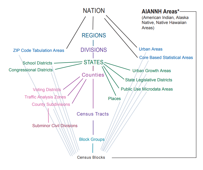
Geography in tidycensus

Information on available geographies, and how to specify them, can be found in the tidycensus documentation
The 2020 Census allows you to get data down to the Census block (unlike the ACS, covered last week)

{width: 400}

Querying by state

For geographies available below the state level, the state parameter allows you to query data for a specific state
tidycensus translates state names and postal abbreviations internally, so you don’t need to remember the FIPS codes!
Example: total population in Missouri by county

mo_population <- get_decennial(
  geography = "county",
  variables = "P1_001N",
  state = "MO",
  sumfile = "dhc",
  year = 2020
)

mo_population

# A tibble: 115 × 4
   GEOID NAME                       variable  value
   <chr> <chr>                      <chr>     <dbl>
 1 29001 Adair County, Missouri     P1_001N   25314
 2 29003 Andrew County, Missouri    P1_001N   18135
 3 29005 Atchison County, Missouri  P1_001N    5305
 4 29007 Audrain County, Missouri   P1_001N   24962
 5 29009 Barry County, Missouri     P1_001N   34534
 6 29011 Barton County, Missouri    P1_001N   11637
 7 29013 Bates County, Missouri     P1_001N   16042
 8 29015 Benton County, Missouri    P1_001N   19394
 9 29017 Bollinger County, Missouri P1_001N   10567
10 29019 Boone County, Missouri     P1_001N  183610
# ℹ 105 more rows

Querying by state and county

County names are also translated internally by tidycensus for sub-county queries, e.g. for Census tracts, block groups, and blocks

stl_blocks <- get_decennial(
  geography = "block",
  variables = "P1_001N",
  state = "MO",
  county = "St. Louis city",
  sumfile = "dhc",
  year = 2020
)

stl_blocks

# A tibble: 8,057 × 4
   GEOID           NAME                                           variable value
   <chr>           <chr>                                          <chr>    <dbl>
 1 295101156001003 Block 1003, Block Group 1, Census Tract 1156,… P1_001N     18
 2 295101156001004 Block 1004, Block Group 1, Census Tract 1156,… P1_001N      0
 3 295101156001005 Block 1005, Block Group 1, Census Tract 1156,… P1_001N     60
 4 295101156001006 Block 1006, Block Group 1, Census Tract 1156,… P1_001N     68
 5 295101156001007 Block 1007, Block Group 1, Census Tract 1156,… P1_001N    566
 6 295101156001008 Block 1008, Block Group 1, Census Tract 1156,… P1_001N      0
 7 295101164004000 Block 4000, Block Group 4, Census Tract 1164,… P1_001N     52
 8 295101164003019 Block 3019, Block Group 3, Census Tract 1164,… P1_001N     51
 9 295101164003020 Block 3020, Block Group 3, Census Tract 1164,… P1_001N    114
10 295101164003021 Block 3021, Block Group 3, Census Tract 1164,… P1_001N     35
# ℹ 8,047 more rows

Searching for variables

To search for variables, use the load_variables() function along with a year and dataset
The View() function in RStudio allows for interactive browsing and filtering

vars <- load_variables(2020, "dhc")

View(vars)

Available decennial Census datasets in tidycensus

The different datasets in the 2020 Census are accessible by specifying a sumfile in get_decennial(). The datasets we’ll cover today include (besides the default PL 94-171 Redistricting Data):

The DHC data (sumfile = "dhc")
The Demographic Profile (sumfile = "dp")
The CD118 data (sumfile = "cd118)
The Detailed DHC-A data (sumfile = "ddhca")
The Detailed DHC-B data (sumfile = "ddhcb")

Data structure in tidycensus

“Tidy” or long-form data

The default data structure returned by tidycensus is “tidy” or long-form data, with variables by geography stacked by row

single_year_age <- get_decennial(
  geography = "state",
  table = "PCT12",
  year = 2020,
  sumfile = "dhc"
)

single_year_age

# A tibble: 10,868 × 4
   GEOID NAME                 variable      value
   <chr> <chr>                <chr>         <dbl>
 1 09    Connecticut          PCT12_001N  3605944
 2 10    Delaware             PCT12_001N   989948
 3 11    District of Columbia PCT12_001N   689545
 4 12    Florida              PCT12_001N 21538187
 5 13    Georgia              PCT12_001N 10711908
 6 15    Hawaii               PCT12_001N  1455271
 7 16    Idaho                PCT12_001N  1839106
 8 17    Illinois             PCT12_001N 12812508
 9 18    Indiana              PCT12_001N  6785528
10 19    Iowa                 PCT12_001N  3190369
# ℹ 10,858 more rows

“Wide” data

The argument output = "wide" spreads Census variables across the columns, returning one row per geographic unit and one column per variable

single_year_age_wide <- get_decennial(
  geography = "state",
  table = "PCT12",
  year = 2020,
  sumfile = "dhc",
  output = "wide" 
)

single_year_age_wide

# A tibble: 52 × 211
   GEOID NAME  PCT12_001N PCT12_002N PCT12_003N PCT12_004N PCT12_005N PCT12_006N
   <chr> <chr>      <dbl>      <dbl>      <dbl>      <dbl>      <dbl>      <dbl>
 1 09    Conn…    3605944    1749853      16946      17489      17974      18571
 2 10    Dela…     989948     476719       4847       5045       5239       5427
 3 11    Dist…     689545     322777       4116       3730       3620       3723
 4 12    Flor…   21538187   10464234      98241     100543     104962     108555
 5 13    Geor…   10711908    5188570      58614      59817      62719      64271
 6 15    Hawa…    1455271     727844       7757       7565       7701       8303
 7 16    Idaho    1839106     919196      11029      10953      11558      12056
 8 17    Illi…   12812508    6283130      68115      69120      71823      74165
 9 18    Indi…    6785528    3344660      39308      40232      41971      43310
10 19    Iowa     3190369    1586092      18038      18566      19349      19864
# ℹ 42 more rows
# ℹ 203 more variables: PCT12_007N <dbl>, PCT12_008N <dbl>, PCT12_009N <dbl>,
#   PCT12_010N <dbl>, PCT12_011N <dbl>, PCT12_012N <dbl>, PCT12_013N <dbl>,
#   PCT12_014N <dbl>, PCT12_015N <dbl>, PCT12_016N <dbl>, PCT12_017N <dbl>,
#   PCT12_018N <dbl>, PCT12_019N <dbl>, PCT12_020N <dbl>, PCT12_021N <dbl>,
#   PCT12_022N <dbl>, PCT12_023N <dbl>, PCT12_024N <dbl>, PCT12_025N <dbl>,
#   PCT12_026N <dbl>, PCT12_027N <dbl>, PCT12_028N <dbl>, PCT12_029N <dbl>, …

Using named vectors of variables

Census variables can be hard to remember; using a named vector to request variables will replace the Census IDs with a custom input
In long form, these custom inputs will populate the variable column; in wide form, they will replace the column names

fl_samesex <- get_decennial(
  geography = "county",
  state = "FL",
  variables = c(married = "DP1_0116P",
                partnered = "DP1_0118P"),
  year = 2020,
  sumfile = "dp",
  output = "wide"
)

fl_samesex

# A tibble: 67 × 4
   GEOID NAME                      married partnered
   <chr> <chr>                       <dbl>     <dbl>
 1 12001 Alachua County, Florida       0.3       0.2
 2 12003 Baker County, Florida         0.1       0.1
 3 12005 Bay County, Florida           0.2       0.2
 4 12007 Bradford County, Florida      0.1       0.1
 5 12009 Brevard County, Florida       0.2       0.1
 6 12011 Broward County, Florida       0.4       0.3
 7 12013 Calhoun County, Florida       0.1       0.1
 8 12015 Charlotte County, Florida     0.2       0.1
 9 12017 Citrus County, Florida        0.2       0.1
10 12019 Clay County, Florida          0.2       0.1
# ℹ 57 more rows

Part 1 exercises

Use load_variables(2020, "dhc") to find a variable that interests you from the Demographic and Housing Characteristics file.
Use get_decennial() to fetch data on that variable from the decennial US Census for counties in a state of your choosing.

Part 2: Analysis workflows with 2020 Census data

The tidyverse

library(tidyverse)

tidyverse_logo()

⬢ __  _    __   .    ⬡           ⬢  . 
 / /_(_)__/ /_ ___  _____ _______ ___ 
/ __/ / _  / // / |/ / -_) __(_-</ -_)
\__/_/\_,_/\_, /|___/\__/_/ /___/\__/ 
     ⬢  . /___/      ⬡      .       ⬢

The tidyverse: an integrated set of packages developed primarily by Hadley Wickham and the Posit team

tidycensus and the tidyverse

Census data are commonly used in wide format, with categories spread across the columns
tidyverse tools work better with data that are in “tidy”, or long format; this format is returned by tidycensus by default
Goal: return data “ready to go” for use with tidyverse tools

Exploring 2020 Census data with tidyverse tools

Finding the largest values

dplyr’s arrange() function sorts data based on values in one or more columns, and filter() helps you query data based on column values
Example: what are the largest and smallest counties in Missouri by population?

library(tidycensus)
library(tidyverse)

mo_population <- get_decennial(
  geography = "county",
  variables = "P1_001N",
  year = 2020,
  state = "MO",
  sumfile = "dhc"
)

arrange(mo_population, value)

# A tibble: 115 × 4
   GEOID NAME                      variable value
   <chr> <chr>                     <chr>    <dbl>
 1 29227 Worth County, Missouri    P1_001N   1973
 2 29129 Mercer County, Missouri   P1_001N   3538
 3 29103 Knox County, Missouri     P1_001N   3744
 4 29197 Schuyler County, Missouri P1_001N   4032
 5 29087 Holt County, Missouri     P1_001N   4223
 6 29171 Putnam County, Missouri   P1_001N   4681
 7 29199 Scotland County, Missouri P1_001N   4716
 8 29035 Carter County, Missouri   P1_001N   5202
 9 29005 Atchison County, Missouri P1_001N   5305
10 29211 Sullivan County, Missouri P1_001N   5999
# ℹ 105 more rows

arrange(mo_population, desc(value))

# A tibble: 115 × 4
   GEOID NAME                         variable   value
   <chr> <chr>                        <chr>      <dbl>
 1 29189 St. Louis County, Missouri   P1_001N  1004125
 2 29095 Jackson County, Missouri     P1_001N   717204
 3 29183 St. Charles County, Missouri P1_001N   405262
 4 29510 St. Louis city, Missouri     P1_001N   301578
 5 29077 Greene County, Missouri      P1_001N   298915
 6 29047 Clay County, Missouri        P1_001N   253335
 7 29099 Jefferson County, Missouri   P1_001N   226739
 8 29019 Boone County, Missouri       P1_001N   183610
 9 29097 Jasper County, Missouri      P1_001N   122761
10 29037 Cass County, Missouri        P1_001N   107824
# ℹ 105 more rows

What are the counties with a population below 5,000?

The filter() function subsets data according to a specified condition, much like a SQL query

below1000 <- filter(mo_population, value < 1000)

below1000

# A tibble: 0 × 4
# ℹ 4 variables: GEOID <chr>, NAME <chr>, variable <chr>, value <dbl>

Using summary variables

Many decennial Census and ACS variables are organized in tables in which the first variable represents a summary variable, or denominator for the others
The parameter summary_var can be used to generate a new column in long-form data for a requested denominator, which works well for normalizing estimates

Using summary variables

race_vars <- c(
  Hispanic = "P5_010N",
  White = "P5_003N",
  Black = "P5_004N",
  Native = "P5_005N",
  Asian = "P5_006N",
  HIPI = "P5_007N"
)

cbsa_race <- get_decennial(
  geography = "cbsa",
  variables = race_vars,
  summary_var = "P5_001N", 
  year = 2020,
  sumfile = "dhc"
)

cbsa_race

# A tibble: 5,634 × 5
   GEOID NAME                                      variable  value summary_value
   <chr> <chr>                                     <chr>     <dbl>         <dbl>
 1 49420 Yakima, WA Metro Area                     Hispanic 130049        256728
 2 49460 Yankton, SD Micro Area                    Hispanic   1234         23310
 3 49500 Yauco, PR Metro Area                      Hispanic  85665         86142
 4 49620 York-Hanover, PA Metro Area               Hispanic  39360        456438
 5 49660 Youngstown-Warren-Boardman, OH-PA Metro … Hispanic  19881        541243
 6 49700 Yuba City, CA Metro Area                  Hispanic  55088        181208
 7 49740 Yuma, AZ Metro Area                       Hispanic 130003        203881
 8 49780 Zanesville, OH Micro Area                 Hispanic   1055         86410
 9 49820 Zapata, TX Micro Area                     Hispanic  12999         13889
10 48300 Wenatchee, WA Metro Area                  Hispanic  36741        122012
# ℹ 5,624 more rows

Normalizing columns with `mutate()`

dplyr’s mutate() function is used to calculate new columns in your data; the select() column can keep or drop columns by name
In a tidyverse workflow, these steps are commonly linked using the pipe operator (%>%) from the magrittr package

cbsa_race_percent <- cbsa_race %>%
  mutate(percent = 100 * (value / summary_value)) %>% 
  select(NAME, variable, percent)

cbsa_race_percent

# A tibble: 5,634 × 3
   NAME                                         variable percent
   <chr>                                        <chr>      <dbl>
 1 Yakima, WA Metro Area                        Hispanic   50.7 
 2 Yankton, SD Micro Area                       Hispanic    5.29
 3 Yauco, PR Metro Area                         Hispanic   99.4 
 4 York-Hanover, PA Metro Area                  Hispanic    8.62
 5 Youngstown-Warren-Boardman, OH-PA Metro Area Hispanic    3.67
 6 Yuba City, CA Metro Area                     Hispanic   30.4 
 7 Yuma, AZ Metro Area                          Hispanic   63.8 
 8 Zanesville, OH Micro Area                    Hispanic    1.22
 9 Zapata, TX Micro Area                        Hispanic   93.6 
10 Wenatchee, WA Metro Area                     Hispanic   30.1 
# ℹ 5,624 more rows

Group-wise Census data analysis

The group_by() and summarize() functions in dplyr are used to implement the split-apply-combine method of data analysis
The default “tidy” format returned by tidycensus is designed to work well with group-wise Census data analysis workflows

What is the largest group by CBSA?

largest_group <- cbsa_race_percent %>%
  group_by(NAME) %>% 
  filter(percent == max(percent)) 

# Optionally, use `.by`: 
# largest_group <- cbsa_race_percent %>%
#   filter(percent == max(percent), .by = NAME)

largest_group

# A tibble: 939 × 3
# Groups:   NAME [939]
   NAME                      variable percent
   <chr>                     <chr>      <dbl>
 1 Yakima, WA Metro Area     Hispanic    50.7
 2 Yauco, PR Metro Area      Hispanic    99.4
 3 Yuma, AZ Metro Area       Hispanic    63.8
 4 Zapata, TX Micro Area     Hispanic    93.6
 5 Del Rio, TX Micro Area    Hispanic    80.3
 6 Deming, NM Micro Area     Hispanic    65.6
 7 Dodge City, KS Micro Area Hispanic    57.4
 8 Dumas, TX Micro Area      Hispanic    59.2
 9 Eagle Pass, TX Micro Area Hispanic    94.9
10 El Centro, CA Metro Area  Hispanic    85.2
# ℹ 929 more rows

What are the median percentages by group?

cbsa_race_percent %>%
  group_by(variable) %>% 
  summarize(median_pct = median(percent, na.rm = TRUE))

# A tibble: 6 × 2
  variable median_pct
  <chr>         <dbl>
1 Asian        1.03  
2 Black        3.61  
3 HIPI         0.0349
4 Hispanic     6.97  
5 Native       0.287 
6 White       75.2

Exploring maps of Census data

“Spatial” Census data

One of the best features of tidycensus is the argument geometry = TRUE, which gets you the correct Census geometries with no hassle
get_decennial() with geometry = TRUE returns a spatial Census dataset containing simple feature geometries; learn more on February 26
Let’s take a look at some examples

“Spatial” Census data

geometry = TRUE does the hard work for you of acquiring and pre-joining spatial Census data
Consider using the Demographic Profile for pre-tabulated percentages

wv_over_65 <- get_decennial(
  geography = "tract",
  variables = "DP1_0024P",
  state = "WV",
  geometry = TRUE,
  sumfile = "dp",
  year = 2020
)

We get back a simple features data frame (more about this on February 26)

wv_over_65

Simple feature collection with 546 features and 4 fields
Geometry type: POLYGON
Dimension:     XY
Bounding box:  xmin: -82.64474 ymin: 37.20148 xmax: -77.71952 ymax: 40.6388
Geodetic CRS:  NAD83
# A tibble: 546 × 5
   GEOID       NAME                     variable value                  geometry
   <chr>       <chr>                    <chr>    <dbl>             <POLYGON [°]>
 1 54001965700 Census Tract 9657; Barb… DP1_002…  22.3 ((-80.07606 39.1016, -80…
 2 54029020700 Census Tract 207; Hanco… DP1_002…  22.4 ((-80.57509 40.41198, -8…
 3 54069000200 Census Tract 2; Ohio Co… DP1_002…  22.3 ((-80.71044 40.12813, -8…
 4 54011001400 Census Tract 14; Cabell… DP1_002…  15.1 ((-82.43736 38.41681, -8…
 5 54099005100 Census Tract 51; Wayne … DP1_002…  23.3 ((-82.54137 38.39631, -8…
 6 54099005200 Census Tract 52; Wayne … DP1_002…  21.8 ((-82.55603 38.39246, -8…
 7 54059957200 Census Tract 9572; Ming… DP1_002…  20.3 ((-82.35141 37.78997, -8…
 8 54071970600 Census Tract 9706; Pend… DP1_002…  29.2 ((-79.47433 38.46251, -7…
 9 54083965900 Census Tract 9659; Rand… DP1_002…  20.1 ((-80.26471 38.71209, -8…
10 54085962400 Census Tract 9624; Ritc… DP1_002…  25   ((-81.32879 39.15258, -8…
# ℹ 536 more rows

Exploring spatial data

Mapping, GIS, and spatial data is the subject of our February 26 workshop - so be sure to check that out!
Even before we dive deeper into spatial data, it is very useful to be able to explore your results on an interactive map
Our solution: mapview()

Exploring spatial data

library(mapview)

mapview(wv_over_65)

Creating a shaded map with `zcol`

mapview(wv_over_65, zcol = "value")

Customizing your mapview output

mapview(wv_over_65, zcol = "value",
        layer.name = "% age 65 and up<br>Census tracts in Iowa")

Customizing your mapview output

library(viridisLite)

mapview(wv_over_65, zcol = "value",
        layer.name = "% age 65 and up<br>Census tracts in W. Virginia",
        col.regions = inferno(100))

Saving and using interactive maps

Use the saveWidget() function over the map slot of your mapview map to save out a standalone HTML file, which you can embed in websites

library(htmlwidgets)

m1 <- mapview(wv_over_65, zcol = "value",
        layer.name = "% age 65 and up<br>Census tracts in W. Virginia",
        col.regions = inferno(100))

saveWidget(m1@map, "wv_over_65.html")

Part 2 exercise

Try making an interactive map of a different variable from the Demographic Profile (use load_variables(2020, "dp") to look them up) for a different state, or state / county combination.

Part 3: The Detailed DHC-A File and time-series analysis

The 2020 Decennial Census Detailed DHC-A File

The Detailed DHC-A File

Tabulation of 2020 Decennial Census results for population by sex and age
Key feature: break-outs for thousands of racial and ethnic groups

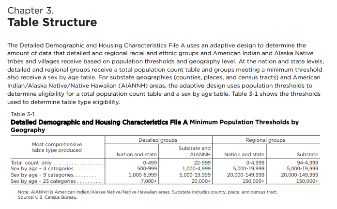
Limitations of the DDHC-A File

An “adaptive design” is used, meaning that data for different groups / geographies may be found in different tables
There is considerable sparsity in the data, especially when going down to the Census tract level

Using the DDHC-A File in tidycensus

You’ll query the DDHC-A file with the argument sumfile = "ddhca" in get_decennial()
A new argument, pop_group, is required to use the DDHC-A; it takes a population group code.
Use pop_group = "all" to query for all groups; set pop_group_label = TRUE to return the label for the population group
Look up variables with load_variables(2020, "ddhca")

Example usage of the DDHC-A File

mn_population_groups <- get_decennial(
  geography = "state",
  variables = "T01001_001N",
  state = "MN",
  year = 2020,
  sumfile = "ddhca",
  pop_group = "all",
  pop_group_label = TRUE
)

mn_population_groups

# A tibble: 2,996 × 6
   GEOID NAME      pop_group pop_group_label   variable      value
   <chr> <chr>     <chr>     <chr>             <chr>         <dbl>
 1 27    Minnesota 1002      European alone    T01001_001N 3162905
 2 27    Minnesota 1003      Albanian alone    T01001_001N     512
 3 27    Minnesota 1004      Alsatian alone    T01001_001N      27
 4 27    Minnesota 1005      Andorran alone    T01001_001N      NA
 5 27    Minnesota 1006      Armenian alone    T01001_001N     605
 6 27    Minnesota 1007      Austrian alone    T01001_001N    2552
 7 27    Minnesota 1008      Azerbaijani alone T01001_001N     103
 8 27    Minnesota 1009      Basque alone      T01001_001N      52
 9 27    Minnesota 1010      Belarusian alone  T01001_001N    1579
10 27    Minnesota 1011      Belgian alone     T01001_001N    3864
# ℹ 2,986 more rows

Looking up group codes

The get_pop_groups(), helps you look up population group codes
It works for SF2/SF4 in 2000 and SF2 in 2010 as well!

available_groups <- get_pop_groups(2020, "ddhca")

Understanding sparsity in the DDHC-A File

The DDHC-A File uses an “adaptive design” that makes certain tables available for specific geographies

You may see this error…

get_decennial(
  geography = "county",
  variables = "T02001_001N",
  state = "MN",
  county = "Hennepin",
  pop_group = "1325",
  year = 2020,
  sumfile = "ddhca"
)

Error in `get_decennial()`:
! Error in load_data_decennial(geography, variables, key, year, sumfile,  : 
  Your DDHC-A request returned No Content from the API.
ℹ The DDHC-A file uses an 'adaptive design' where data availability varies by geography and by population group.
ℹ Read Section 3-1 at https://www2.census.gov/programs-surveys/decennial/2020/technical-documentation/complete-tech-docs/detailed-demographic-and-housing-characteristics-file-a/2020census-detailed-dhc-a-techdoc.pdf for more information.
ℹ In tidycensus, use the function `check_ddhca_groups()` to see if your data is available.

How to check for data availability

The function check_ddhca_groups(), can be used to see which tables to use for the data you want

check_ddhca_groups(
  geography = "county", 
  pop_group = "1325", 
  state = "MN", 
  county = "Hennepin"
)

Mapping DDHC-A data

Given data sparsity in the DDHC-A data, should you make maps with it?
I’m not personally a fan of mapping data that are geographically sparse. But…

I think it is OK to map DDHC-A data if you think through the data limitations in your map design

Example: Somali populations by Census tract in Minneapolis

library(tidycensus)

hennepin_somali <- get_decennial(
  geography = "tract",
  variables = "T01001_001N",
  state = "MN",
  county = "Hennepin",
  year = 2020,
  sumfile = "ddhca",
  pop_group = "1325",
  pop_group_label = TRUE,
  geometry = TRUE
)

mapview(hennepin_somali, zcol = "value")

Alternative approach: dot-density mapping

I don’t think choropleth maps are advisable with geographically incomplete data in most cases
Other map types - like graduated symbols or dot-density maps - may be more appropriate
The tidycensus function as_dot_density() allows you to specify the number of people represented in each dot, which means you can represent data-suppressed areas as 0 more confidently

somali_dots <- as_dot_density(
  hennepin_somali,
  value = "value",
  values_per_dot = 25
)

mapview(somali_dots, cex = 0.01, layer.name = "Somali population<br>1 dot = 25 people",
        col.regions = "navy", color = "navy")

Time-series analysis

How have areas changed since the 2010 Census?

A common use-case for the 2020 decennial Census data is to assess change over time
For example: which areas have experienced the most population growth, and which have experienced the steepest declines?
tidycensus allows users to access the 2000 and 2010 decennial Census data for comparison, though variable IDs will differ

Getting data from the 2010 Census

county_pop_10 <- get_decennial(
  geography = "county",
  variables = "P001001", 
  year = 2010,
  sumfile = "sf1"
)

county_pop_10

# A tibble: 3,221 × 4
   GEOID NAME                        variable  value
   <chr> <chr>                       <chr>     <dbl>
 1 05131 Sebastian County, Arkansas  P001001  125744
 2 05133 Sevier County, Arkansas     P001001   17058
 3 05135 Sharp County, Arkansas      P001001   17264
 4 05137 Stone County, Arkansas      P001001   12394
 5 05139 Union County, Arkansas      P001001   41639
 6 05141 Van Buren County, Arkansas  P001001   17295
 7 05143 Washington County, Arkansas P001001  203065
 8 05145 White County, Arkansas      P001001   77076
 9 05149 Yell County, Arkansas       P001001   22185
10 06011 Colusa County, California   P001001   21419
# ℹ 3,211 more rows

Cleanup before joining

The select() function can both subset datasets by column and rename columns, “cleaning up” a dataset before joining to another dataset

county_pop_10_clean <- county_pop_10 %>%
  select(GEOID, value10 = value) 

county_pop_10_clean

# A tibble: 3,221 × 2
   GEOID value10
   <chr>   <dbl>
 1 05131  125744
 2 05133   17058
 3 05135   17264
 4 05137   12394
 5 05139   41639
 6 05141   17295
 7 05143  203065
 8 05145   77076
 9 05149   22185
10 06011   21419
# ℹ 3,211 more rows

Joining data

In dplyr, joins are implemented with the *_join() family of functions

county_pop_20 <- get_decennial(
  geography = "county",
  variables = "P1_001N",
  year = 2020,
  sumfile = "dhc"
) %>%
  select(GEOID, NAME, value20 = value)

county_joined <- county_pop_20 %>%
  left_join(county_pop_10_clean, by = "GEOID")

county_joined

# A tibble: 3,221 × 4
   GEOID NAME                         value20 value10
   <chr> <chr>                          <dbl>   <dbl>
 1 06039 Madera County, California     156255  150865
 2 06041 Marin County, California      262321  252409
 3 06043 Mariposa County, California    17131   18251
 4 06045 Mendocino County, California   91601   87841
 5 06047 Merced County, California     281202  255793
 6 06049 Modoc County, California        8700    9686
 7 06051 Mono County, California        13195   14202
 8 06053 Monterey County, California   439035  415057
 9 06055 Napa County, California       138019  136484
10 06057 Nevada County, California     102241   98764
# ℹ 3,211 more rows

Calculating change

dplyr’s mutate() function can be used to calculate new columns, allowing for assessment of change over time

county_change <- county_joined %>%
  mutate( 
    total_change = value20 - value10, 
    percent_change = 100 * (total_change / value10) 
  )

county_change

# A tibble: 3,221 × 6
   GEOID NAME                        value20 value10 total_change percent_change
   <chr> <chr>                         <dbl>   <dbl>        <dbl>          <dbl>
 1 06039 Madera County, California    156255  150865         5390           3.57
 2 06041 Marin County, California     262321  252409         9912           3.93
 3 06043 Mariposa County, California   17131   18251        -1120          -6.14
 4 06045 Mendocino County, Californ…   91601   87841         3760           4.28
 5 06047 Merced County, California    281202  255793        25409           9.93
 6 06049 Modoc County, California       8700    9686         -986         -10.2 
 7 06051 Mono County, California       13195   14202        -1007          -7.09
 8 06053 Monterey County, California  439035  415057        23978           5.78
 9 06055 Napa County, California      138019  136484         1535           1.12
10 06057 Nevada County, California    102241   98764         3477           3.52
# ℹ 3,211 more rows

Caveat: changing geographies!

County names and boundaries can change from year to year, introducing potential problems in time-series analysis
This is particularly acute for small geographies like Census tracts & block groups, which we’ll cover on February 26!

filter(county_change, is.na(value10))

# A tibble: 4 × 6
  GEOID NAME                         value20 value10 total_change percent_change
  <chr> <chr>                          <dbl>   <dbl>        <dbl>          <dbl>
1 02063 Chugach Census Area, Alaska     7102      NA           NA             NA
2 02066 Copper River Census Area, A…    2617      NA           NA             NA
3 02158 Kusilvak Census Area, Alaska    8368      NA           NA             NA
4 46102 Oglala Lakota County, South…   13672      NA           NA             NA

Need data before 2000? Use NHGIS

Working with Decennial Census Data in R

About me

SSDAN webinar series

Today’s agenda

Getting started with 2020 Decennial US Census data in R

R and RStudio

What is the decennial US Census?

The 2020 US Census: available datasets

How to get decennial Census data

tidycensus

tidycensus: key features

Getting started with tidycensus

Optional: your Census API key

Getting started with Census data in tidycensus

2020 Census data in tidycensus

Understanding the printed messages

Understanding the printed messages

Requesting tables of variables

US Census Geography

Geography in tidycensus

Querying by state

Querying by state and county

Searching for variables

Available decennial Census datasets in tidycensus

Data structure in tidycensus

“Tidy” or long-form data

“Wide” data

Using named vectors of variables

Part 1 exercises

Part 2: Analysis workflows with 2020 Census data

The tidyverse

tidycensus and the tidyverse

Exploring 2020 Census data with tidyverse tools

Finding the largest values

What are the counties with a population below 5,000?

Using summary variables

Using summary variables

Normalizing columns with mutate()

Group-wise Census data analysis

What is the largest group by CBSA?

What are the median percentages by group?

Exploring maps of Census data

“Spatial” Census data

“Spatial” Census data

Exploring spatial data

Exploring spatial data

Creating a shaded map with zcol

Customizing your mapview output

Customizing your mapview output

Saving and using interactive maps

Part 2 exercise

Part 3: The Detailed DHC-A File and time-series analysis

The 2020 Decennial Census Detailed DHC-A File

The Detailed DHC-A File

Limitations of the DDHC-A File

Using the DDHC-A File in tidycensus

Example usage of the DDHC-A File

Looking up group codes

Understanding sparsity in the DDHC-A File

You may see this error…

How to check for data availability

Mapping DDHC-A data

Example: Somali populations by Census tract in Minneapolis

Alternative approach: dot-density mapping

Time-series analysis

How have areas changed since the 2010 Census?

Getting data from the 2010 Census

Cleanup before joining

Joining data

Calculating change

Caveat: changing geographies!

Need data before 2000? Use NHGIS

Thank you!

Normalizing columns with `mutate()`

Creating a shaded map with `zcol`