Point clustering

Let’s make a map of US power plants where each cluster is a donut chart showing the mix of fuel types. freestiler builds the clusters and category counts into PMTiles; mapgl draws the donuts from those tile properties. The browser only downloads the tiles in view.

This example uses the Global Power Plant Database from the World Resources Institute and partners, licensed under CC BY 4.0. The download is pinned to a snapshot of version 1.3.0. It is a historical inventory, not a current list of operating plants. Each point counts as one plant, regardless of capacity.

US power plants grouped into donut clusters by primary fuel.

Install the packages

This R example requires freestiler 0.3.0.9000 or later from R-Universe and mapgl 0.5.2 or later. CRAN 0.3.0 does not support categorical clustering directly from sf objects. The implementation is compatible with the CRAN build and will be included in the next CRAN release. Restart R before replacing an existing installation:

install.packages(
  "freestiler",
  repos = c("https://walkerke.r-universe.dev", "https://cloud.r-project.org")
)
install.packages(c("mapgl", "sf", "jsonlite", "httpuv"))

Run the following sections in order in the same R session. We will read the data into an sf object and pass it directly to freestile(). No API key is required.

Download and prepare the points

library(sf)
library(freestiler)
library(mapgl)

dir.create("power-plant-demo", showWarnings = FALSE)
csv_path <- "power-plant-demo/power-plants.csv"
data_url <- paste0(
  "https://raw.githubusercontent.com/wri/global-power-plant-database/",
  "7a91cfbb2a4e272597acbc00506d61fc1ec73b3d/",
  "output_database/global_power_plant_database.csv"
)
download.file(data_url, csv_path, mode = "wb")
plants <- read.csv(csv_path)

# Keep the contiguous US and the attributes used in the map.
plants <- subset(
  plants,
  country == "USA" & longitude > -126 & longitude < -66 &
    latitude > 24 & latitude < 50,
  select = c(gppd_idnr, name, primary_fuel, longitude, latitude)
)
plants <- plants[order(plants$gppd_idnr), ]
fuels <- c("Solar", "Wind", "Hydro", "Gas", "Coal", "Nuclear", "Other")
plants$fuel <- ifelse(plants$primary_fuel %in% fuels, plants$primary_fuel, "Other")
plants <- st_as_sf(plants, coords = c("longitude", "latitude"), crs = 4326)

This leaves 9,581 plants. Sorting by plant ID fixes the input order, which matters for reproducible cluster membership. The fuel groups and their order will be shared by the tiler, the donut charts, and the legend.

Build the tiles

freestile(
  plants,
  "power-plant-demo/plants.pmtiles",
  layer_name = "plants",
  min_zoom = 0,
  max_zoom = 14,
  cluster_distance = 60,
  cluster_maxzoom = 9,
  category = "fuel",
  category_values = fuels
)

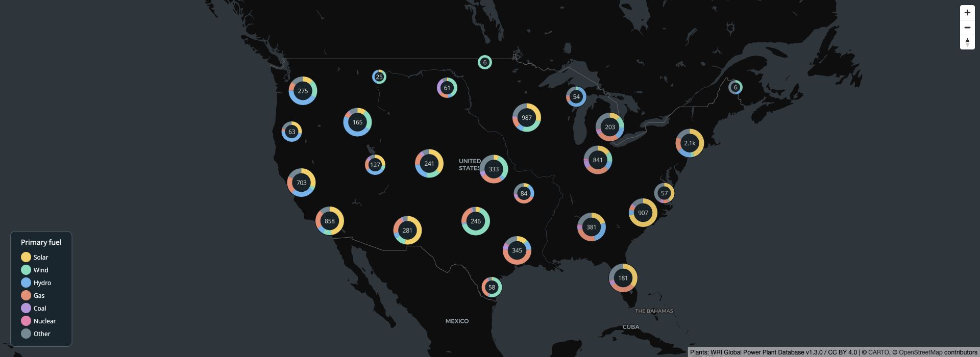
The archive contains clusters through zoom 9 and individual plants from zoom 10 onward. Every cluster carries point_count and counts named fuel:Solar, fuel:Wind, and so on. These are plant counts, not megawatts or electricity generation. Isolated plants retain their name and other original attributes.

Draw donut charts with mapgl

colors <- c("#f9cf58", "#71debd", "#64b5ee", "#f18c70", "#bb95df", "#ef7daf", "#728a94")
fuel_color <- match_expr("fuel", values = fuels, stops = colors, default = "#728a94")

# Keep this R session running while viewing the map.
serve_tiles("power-plant-demo", port = 8082)

plant_map <- maplibre(
  style = carto_style("dark-matter"),
  center = c(-98, 38.5), zoom = 3.5,
  projection = "mercator", height = 700,
  attributionControl = list(customAttribution = "Plants: WRI Global Power Plant Database v1.3.0 / CC BY 4.0")
) |>
  add_pmtiles_source(
    "plant-source", "http://localhost:8082/plants.pmtiles", maxzoom = 14
  ) |>
  add_circle_layer(
    "plants", source = "plant-source", source_layer = "plants",
    circle_color = fuel_color, circle_radius = 4,
    popup = "name",
    cluster_options = cluster_options(
      max_zoom = 9,
      donut_column = "fuel", donut_values = fuels, donut_colors = colors,
      radius_stops = c(14, 20, 28), count_stops = c(0, 30, 150),
      donut_width = 0.35, donut_fill = "#142329", text_color = "#f6f4e9",
      circle_stroke_color = "#10191e"
    )
  ) |>
  add_categorical_legend(
    "Primary fuel", values = fuels, colors = colors,
    position = "bottom-left", patch_shape = "circle",
    style = legend_style(
      background_color = "#16262e", text_color = "#e7efef",
      title_color = "white", border_color = "#52616a"
    )
  ) |>
  add_navigation_control()

plant_map

The number inside each donut is the number of plants. Its slices show their fuel mix. Because source names a PMTiles source, mapgl uses the clusters freestiler already computed. Passing an sf object as source would instead ask the browser to cluster the points.

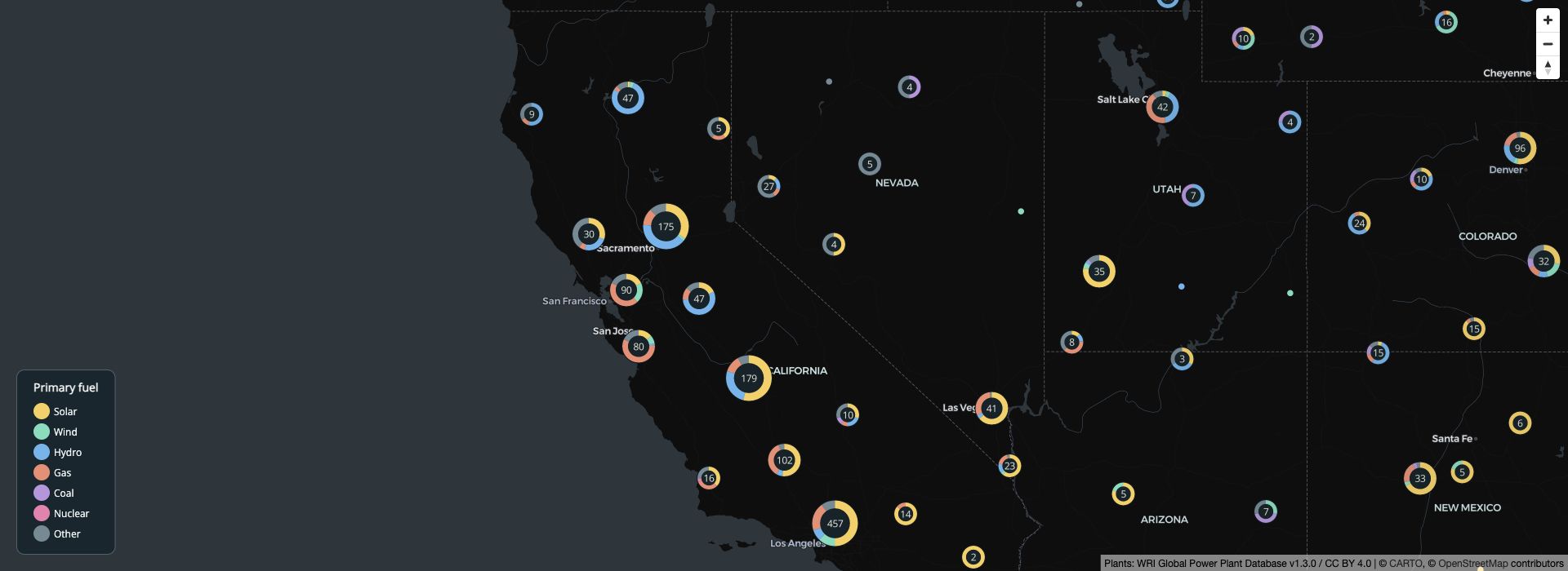
Zoom in to see the regional differences. At zoom 10 the clusters give way to individual plants from the same archive. Click a plant to see its name.

set_view(plant_map, center = c(-119, 38), zoom = 5.5)

A closer view of power plants in the western US, with smaller donut clusters and individual plants.

When finished, stop the tile server with stop_server(port = 8082).

Build the same clusters in Python

In Python, read the data into a GeoDataFrame and pass it to freestile() in the same way. This requires freestiler 0.3.1.dev0 or later; PyPI 0.3.0 does not support categorical clustering directly from GeoDataFrames. Until the next PyPI release, install the development version from GitHub (building from source requires Rust):

pip install "git+https://github.com/walkerke/freestiler.git#subdirectory=python"

from pathlib import Path
import pandas as pd
import geopandas as gpd
from freestiler import freestile

folder = Path("power-plant-demo")
folder.mkdir(exist_ok=True)
data_url = (
    "https://raw.githubusercontent.com/wri/global-power-plant-database/"
    "7a91cfbb2a4e272597acbc00506d61fc1ec73b3d/"
    "output_database/global_power_plant_database.csv"
)
plants = pd.read_csv(data_url, low_memory=False)
plants = plants.loc[
    (plants.country == "USA") & plants.longitude.between(-126, -66, inclusive="neither")
    & plants.latitude.between(24, 50, inclusive="neither"),
    ["gppd_idnr", "name", "primary_fuel", "longitude", "latitude"],
].sort_values("gppd_idnr")
fuels = ["Solar", "Wind", "Hydro", "Gas", "Coal", "Nuclear", "Other"]
plants["fuel"] = plants.primary_fuel.where(plants.primary_fuel.isin(fuels), "Other")
plants = gpd.GeoDataFrame(
    plants, geometry=gpd.points_from_xy(plants.longitude, plants.latitude), crs=4326
).drop(columns=["longitude", "latitude"])

freestile(
    plants, folder / "plants.pmtiles",
    layer_name="plants", min_zoom=0, max_zoom=14,
    cluster_distance=60, cluster_maxzoom=9,
    category="fuel", category_values=fuels,
)

This archive can be viewed with the R map code above; load freestiler and mapgl and define fuels first. The Python article also covers serving PMTiles for other viewers.

Properties in the tiles

Property	Meaning
cluster	true for a cluster; absent on a singleton.
cluster_id	Identifier for a cluster.
point_count	Total number of input points in the cluster.
point_count_abbreviated	Abbreviated count for labels, such as "1.2k".
cluster_expansion_zoom	Zoom level where the cluster splits, useful for click-to-zoom.
fuel:Solar, fuel:Wind, etc.	Counts for the declared categories.
fuel:_other	Count of missing or unlisted categories.

The category counts sum to point_count. Divide a category count by point_count to calculate its share. Singletons retain their original attributes and category counts, but have no point_count property. Clusters do not inherit an arbitrary member’s attributes, such as its name.

The example explicitly groups less common fuels into "Other", so those counts live in fuel:Other. The separate fuel:_other field is for values outside the declared dictionary. Zero-count categories are retained.

Zooms and memory

Categorical clustering uses Supercluster 8.0.1 with a 512-pixel tile extent. It accepts a single POINT sf object or GeoDataFrame and a dictionary of 1 to 64 distinct strings or whole numbers. Input is reprojected to WGS84 as needed. Changing row order can change cluster membership.

Use cluster_maxzoom to choose the last zoom with clusters. Individual points fill the remaining zooms through max_zoom. Keep base_zoom unset and simplification at its default, and omit drop_rate and coalesce so all points contribute to the counts.

The input and global clustering index stay in memory. Tile output and singleton attributes are stored on disk, but this is not the streaming query pipeline. The input must contain fewer than 2^31 rows. Select only the properties you need.

For data already stored in GeoParquet, freestile_file() also supports categories in the released 0.3.0 packages. That path requires native GeoParquet support (R-Universe or Python), WGS84 POINT input, and cluster_maxzoom = max_zoom; it currently writes clustered zooms only.

For summaries on a fixed grid, including the most common category and its share, use H3 binning.