Dynamic web maps with Mapbox Tiling Service and mapgl
Source:vignettes/dynamic-maps.Rmd
dynamic-maps.Rmdmapboxapi version 0.5 added support for the Mapbox Tiling Service (MTS) API, Mapbox’s recommended tool for publishing and maintaining vector tile data pipelines. A major benefit to using R and mapboxapi to interact with MTS is that data pipelines for web maps can be handled directly from R. This vignette covers an example walkthrough of how to build dynamic web maps with vector tiles using Mapbox Tiling Service and the mapgl R package, a flexible R interface to Mapbox GL JS.
Warning: Using MTS is not free, and large tileset processing jobs (like this one) that cover a large extent can incur significant charges to your Mapbox account. Please use with caution.
We’ll be making a map of household access to a broadband internet subscription from the 2016-2020 American Community Survey that varies by zoom level. The map should show county broadband internet access when zoomed out, and Census tract level information when zoomed in. We will accomplish this by preparing a multi-layer tileset that will store information for both aggregation levels.
To get started, let’s grab some data from the US Census Bureau using tidycensus. This example assumes you have a Census API key; review the tidycensus documentation to get set up if you don’t.
library(tidycensus)
library(mapboxapi)

county_broadband <- get_acs(
  geography = "county",
  variables = "DP02_0154P",
  year = 2020,
  geometry = TRUE
)

tract_broadband <- get_acs(
  geography = "tract",
  variables = "DP02_0154P",
  state = c(state.abb, "DC"),
  year = 2020,
  geometry = TRUE
)
Publishing vector tiles from R with Mapbox Tiling Service
Spatial data prepared in R can be published to a user’s Mapbox account with just a few steps. These steps involve creating tileset sources, which are datasets stored as raw GeoJSON in a user’s account; preparing a tileset recipe, which tells Mapbox how to create vector tiles from the GeoJSON sources; then creating and publishing vector tilesets. These vector tilesets can be integrated directly into maps with Mapbox GL JS / the mapboxer R package, or added to Mapbox styles using Mapbox Studio.
To create tileset sources directly from R, we using the function
mts_create_source(). We’ll create a source for each dataset
that we want to include in our tileset. Assigning the results of
mts_create_source() to an object allows us to capture the
function’s list output, which will be useful when building the tileset
recipe.
mts_create_source() requires a Mapbox access token with
secret scope and write access to your Mapbox account. Visit
the Mapbox website for more information about access tokens, and
store yours using the mb_access_token() function. You’ll
also supply your own username to the username argument,
rather than use mine. Large datasets can take a few minutes to upload to
your account depending on your connection speed.
county_source <- mts_create_source(
  data = county_broadband,
  tileset_id = "county_broadband",
  username = "kwalkertcu"
)

tract_source <- mts_create_source(
  data = tract_broadband,
  tileset_id = "tract_broadband",
  username = "kwalkertcu"
)
If the upload has succeeded, you’ll get a message like this:
✔ Successfully created tileset source with the ID
'mapbox://tileset-source/kwalkertcu/tract_broadband'.
Use your source ID to build your tileset's recipe.
The tileset ID is also stored in the id element of the
returned list. If your request has failed, you should get an error
message telling you why.
You’ll now use these tileset IDs to prepare a recipe. MTS recipes are JSON documents that translate tileset sources to vector tiles. Preparing a recipe using the MTS documentation can be complicated as there are many options, but mapboxapi tries to simplify this process a bit:
-
mts_make_recipe()is the general “recipe creation” function that takes one or more recipe layers and formats their configuration appropriately for the MTS API. - Recipe layers can be prepared as an R list by hand, or preferably
with the
recipe_layer()function which helps users understand the range of options available. Feature- and tile- specific options are available infeature_options()andtile_options(), respectively.
- Some translation of the JSON examples provided by Mapbox and R’s
notation will be necessary. When reading through the MTS documentation,
remember the following:
- A named list will be translated to a JSON object (curly braces);
- An unnamed list will be translated to a JSON array (square brackets).
Our recipe will include two layers (counties and tracts). A recipe
layer requires a tileset source ID, a minimum zoom level
(minzoom), and maximum zoom level
(maxzoom).
broadband_recipe <- mts_make_recipe(
  counties = recipe_layer(
    source = county_source$id,
    minzoom = 2,
    maxzoom = 7
  ),
  tracts = recipe_layer(
    source = tract_source$id,
    minzoom = 7,
    maxzoom = 12,
    tiles = tile_options(
      layer_size = 2500
    )
  )
)
Our recipe is relatively simple, as MTS recipes are concerned; we include the required arguments (though layers can be viewed beyond the maximum zoom level with overzooming) as well as directions to max out the layer size for our tracts, ensuring that we can see as many tracts as possible when zoomed out.
After preparing an MTS recipe, it can be passed to the
mts_validate_recipe() function to make sure that it is
formatted correctly.
mts_validate_recipe(broadband_recipe)We get the message ✔ Your tileset recipe is valid!; the
function also returns TRUE or FALSE so you can
do error handling in tileset creation pipelines if you wish.
Just two more steps are required to publish the new tileset. We
create the tileset with mts_create_tileset():
mts_create_tileset(
  tileset_name = "us_broadband",
  username = "kwalkertcu",
  recipe = broadband_recipe
)
An empty tileset will be created in our Mapbox account. To populate
the tileset, publish it with mts_publish_tileset()
mts_publish_tileset(
tileset_name = "us_broadband",
username = "kwalkertcu"
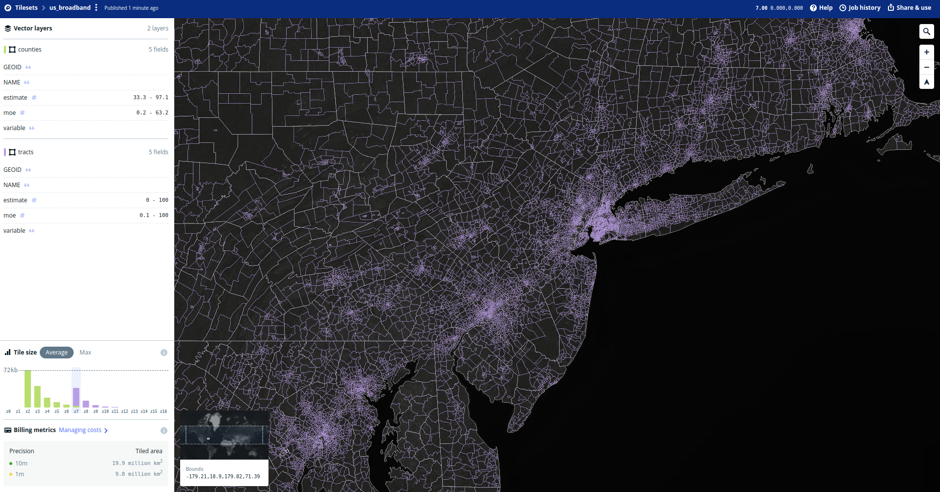
)To check on the status of your tileset, you can head over to your Mapbox account and find your tileset on the Tilesets tab. Once the tileset is published, you’ll be able to browse your tileset and review its recipe.
Using vector tilesets in R with the mapgl package
The mapgl R package is a a flexible R interface to Mapbox GL JS, Mapbox’s JavaScript web mapping library with a massive amount of features. mapboxapi and mapgl work quite nicely together; mapboxapi can handle the creation and maintenance of vector tileset pipelines, and mapgl then handles the visualization of those tiles.
The add_vector_source() function in mapgl allows users
to load remote vector tile sources from their Mapbox account; the
add_fill_layer() function then helps users add layers from
those tileset sources. Given that we’ve already tiled our county and
tract data, we can visualize all 3000+ US counties and all 80,000+
Census tracts intelligently on the same map.
The code used below (click “Show code” to view it) uses mapgl to visualize counties and Census tracts in a scale-dependent manner. At small zooms (below 7), counties will display; at larger zooms (7 and up), the view will switch over to Census tracts.
library(mapgl)

mapboxgl(style = mapbox_style("light"),
         zoom = 3,
         center = c(-96, 37.5)) |>
  add_vector_source(
    id = "broadband",
    url = "mapbox://kwalkertcu.us_broadband"
  ) |>
  add_fill_layer(
    id = "county",
    source = "broadband",
    source_layer = "counties",
    fill_color = "blue",
    fill_outline_color = "black",
    fill_opacity = 0.5,
    max_zoom = 7
  ) |>
  add_fill_layer(
    id = "tracts",
    source = "broadband",
    source_layer = "tracts",
    fill_color = "red",
    fill_outline_color = "black",
    fill_opacity = 0.5,
    min_zoom = 7
  )
Styling vector tiles with Mapbox GL JS and mapgl
Mapbox GL JS has many, many more options available for users to customize styling of their vector tiles. While those options are voluminous, mapgl includes a variety of helper functions to assist with styling.
The example below modifies the map using the following options:
- An Albers projection appropriate for the United States is used
instead of the default Globe projection.
- Counties and Census tracts are styled using linear interpolation
with the
interpolate()function inspired by the ColorBrewer YlGnBU palette. - For Census tracts, the
"case"option is used forNAvalues to make tracts missing data mostly transparent.
broadband_map <- mapboxgl(style = mapbox_style("light"),
         zoom = 3,
         center = c(-96, 37.5),
         projection = "albers",
         parallels = c(29.5, 45.5)) |>
  add_vector_source(
    id = "broadband",
    url = "mapbox://kwalkertcu.us_broadband"
  ) |>
  add_fill_layer(
    id = "county",
    source = "broadband",
    source_layer = "counties",
    fill_color = interpolate(
      column = "estimate",
      values = c(33, 65, 97),
      stops = c("#edf8b1", "#7fcdbb", "#2c7fb8")
    ),
    fill_opacity = 0.5,
    max_zoom = 7,
    popup = "estimate",
    hover_options = list(
      fill_color = "cyan",
      fill_opacity = 1
    )
  ) |>
  add_fill_layer(
    id = "tracts",
    source = "broadband",
    source_layer = "tracts",
    fill_color = interpolate(
      column = "estimate",
      values = c(33, 65, 97),
      stops = c("#edf8b1", "#7fcdbb", "#2c7fb8"),
      na_color = "white"
    ),
    fill_opacity = 0.5,
    min_zoom = 7,
    popup = "estimate",
    hover_options = list(
      fill_color = "cyan",
      fill_opacity = 1
    )
  )

broadband_map
Adding a custom-built legend
While the map data are styled in relationship to locations’ broadband
access, we’ll also want to add a legend to our map to communicate the
information to our viewers more clearly. The add_legend()
function in mapgl accommodates both continuous legends (the default,
which we’ll use here) along with categorical legends.