In Chapter 11 of my book Analyzing US Census Data, I explore a sampling of the variety of government datasets that are available for the United States. One of the most useful of these datasets is LODES (LEHD Origin-Destination Employment Statistics). LODES is a synthetic dataset that represents, down to the Census block level, job counts by workplace and residence as well as the flows between them.
Given that LODES data are tabulated at the Census block level, analysts will often want to merge the data to Census geographic data like what is accessible in the pygris package. pygris includes a function, get_lodes(), that is modeled after the excellent lehdr R package by Jamaal Green, Dillon Mahmoudi, and Liming Wang.
This post will illustrate how to analyze the origins of commuters to the Census tract containing Apple’s headquarters in Cupertino, CA. In doing so, I’ll highlight some of the data wrangling utilities in pandas that allow for the use of method chaining, and show how to merge data to pygris shapes for mapping. The corresponding section in Analyzing US Census Data to this post is “Analyzing labor markets with lehdr.”
Acquiring and wrangling LODES data
To get started, let’s import the functions and modules we need and give get_lodes() a try. get_lodes() requires specifying a state (as state abbreviation) and year; we are getting data for California in 2019, the most recent year currently available. The argument lodes_type = "od" tells pygris to get origin-destination flows data, and cache = True will download the dataset (which is nearly 100MB) to a local cache directory for faster use in the future.
from pygris import tracts from pygris.data import get_lodesimport matplotlib.pyplot as pltca_lodes_od = get_lodes( state ="CA", year =2019, lodes_type ="od", cache =True)ca_lodes_od.head()
w_geocode
h_geocode
S000
SA01
SA02
SA03
SE01
SE02
SE03
SI01
SI02
SI03
createdate
0
060014001001007
060014001001044
1
0
0
1
0
0
1
0
0
1
20211018
1
060014001001007
060014001001060
1
0
0
1
0
0
1
0
0
1
20211018
2
060014001001007
060014038002002
1
1
0
0
1
0
0
0
0
1
20211018
3
060014001001007
060014041021003
1
0
1
0
0
0
1
0
0
1
20211018
4
060014001001007
060014042002012
1
0
0
1
0
1
0
0
0
1
20211018
The loaded dataset, which has nearly 16 million rows, represents synthetic origin-destination flows from Census block to Census block in California in 2019. Columns represent the Census block GEOIDs for both workplace and residence, as well as job counts for flows between them. S000 represents all jobs; see the LODES documentation for how other breakouts are defined.
16 million rows is a lot of data to deal with all at once, so we’ll want to do some targeted data wrangling to make this more manageable. We’ll do so using a method chain, which is my preferred way to do data wrangling in Python given that I come from an R / tidyverse background. The code takes the full origin-destination dataset, rolls it up to the Census tract level, then returns (by Census tract) the number of commuters to Apple’s Census tract in Cupertino.
The .assign() method is used to calculate two new Census tract columns. A great thing about Census GEOIDs is that child geographies (like Census blocks) contain information about parent geographies. In turn, we can calculate Census tract GEOIDs by slicing block GEOIDs for the first 11 characters.
.query() is used to subset our data. We only want rows representing commuters to the Apple campus (or the area around it), so we query for that specific tract ID.
Next, we’ll roll up our data to the tract level. We’ll first group the data by home Census tract with .groupby(), then calculate group sums with .agg().
Finally, we use a dictionary passed to .rename() to give the jobs column a more interpretable name.
Next, we’ll repeat this process to tabulate the total number of workers by home Census tract to be used as a denominator. After that, we can merge the Apple-area commuters dataset back in, and calculate a rate per 1000. Note the lambda notation used in the final step of the method chain: this allows us to refer to the dataset that is being created by the chain.
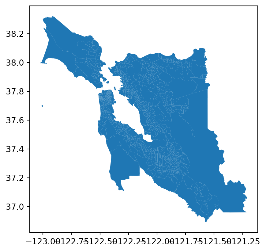
The main purpose of the pygris package is to make the acquisition of US Census Bureau spatial data easy for Python users. Given that we have aggregated our data at the Census tract level, we can use the tracts() function to grab Census tract shapes for six counties in the San Francisco Bay Area. We’ll use the Cartographic Boundary shapefiles with cb = True to exclude most water area, and make sure to specify year = 2019 to match the 2019 LODES data.
Using FIPS code '075' for input 'San Francisco'
Using FIPS code '001' for input 'Alameda'
Using FIPS code '081' for input 'San Mateo'
Using FIPS code '085' for input 'Santa Clara'
Using FIPS code '041' for input 'Marin'
Using FIPS code '013' for input 'Contra Costa'
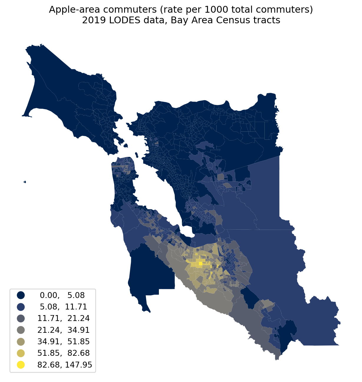
apple_bay = bay_tracts.merge(apple_commuters, left_on ="GEOID", right_on ="h_tract", how ="left")apple_bay.fillna(0, inplace =True)apple_bay.plot(column ='apple_per_1000', legend =True, cmap ="cividis", figsize = (8, 8), k =7, scheme ="naturalbreaks", legend_kwds = {"loc": "lower left"})plt.title("Apple-area commuters (rate per 1000 total commuters)\n2019 LODES data, Bay Area Census tracts", fontsize =12)ax = plt.gca()ax.set_axis_off()
Commuters to Apple’s tract tend to be concentrated around that tract; however, several neighborhoods in San Francisco proper send dozens of commuters per 1000 total commuters south to Cupertino.
This is where the LODES section of my book chapter ends; however, a static map like this can be difficult to interpret for those less familiar with the Bay Area. The geopandas.explore() method can make this map interactive for exploration without much more code. We’ll also use the built-in Census geocoding interface in pygris to add a marker where Apple Park’s visitors center is located.
from pygris.geocode import geocodeapple_bay_sub = apple_bay.filter(['GEOID', 'total_workers','apple_workers', 'apple_per_1000','geometry'])visitor_center = geocode("10600 N Tantau Ave, Cupertino, CA 95014", as_gdf =True)m = apple_bay_sub.explore(column ="apple_per_1000", cmap ="cividis", k =7, scheme ="naturalbreaks", popup =True, tooltip =False, tiles ="CartoDB positron", style_kwds = {"weight": 0.5}, legend_kwds = {"caption": "Apple-area commuters per 1000","colorbar": False}, popup_kwds = {"aliases": ['Census tract', 'Total workers','Apple-area commuters', 'Rate per 1000']})visitor_center.explore(m = m, marker_type ="marker", tooltip =False)
Make this Notebook Trusted to load map: File -> Trust Notebook
If you’ve found this post useful, follow along on Twitter, LinkedIn, or subscribe to my newsletter for more examples of how to translate topics from my book to Python in advance of the book’s release next month!