2 An introduction to tidycensus
The tidycensus package (K. Walker and Herman 2021), first released in 2017, is an R package designed to facilitate the process of acquiring and working with US Census Bureau population data in the R environment. The package has two distinct goals. First, tidycensus aims to make Census data available to R users in a tidyverse-friendly format, helping kick-start the process of generating insights from US Census data. Second, the package is designed to streamline the data wrangling process for spatial Census data analysts. With tidycensus, R users can request geometry along with attributes for their Census data, helping facilitate mapping and spatial analysis. This functionality of tidycensus is covered in more depth in Chapters 6, 7, and 8.
As discussed in the previous chapter, the US Census Bureau makes a wide range of datasets available to the user community through their APIs and other data download resources. tidycensus is not a comprehensive portal to these data resources; instead, it focuses on a select number of datasets implemented in a series of core functions. These core functions in tidycensus include:
get_decennial(), which requests data from the US Decennial Census APIs for 2000, 2010, and 2020.get_acs(), which requests data from the 1-year and 5-year American Community Survey samples. Data are available from the 1-year ACS back to 2005 and the 5-year ACS back to 2005-2009.get_estimates(), an interface to the Population Estimates APIs. These datasets include yearly estimates of population characteristics by state, county, and metropolitan area, along with components of change demographic estimates like births, deaths, and migration rates.get_pums(), which accesses data from the ACS Public Use Microdata Sample APIs. These samples include anonymized individual-level records from the ACS organized by household and are highly useful for many different social science analyses.get_pums()is covered in more depth in Chapters 9 and 10.get_flows(), an interface to the ACS Migration Flows APIs. Includes information on in- and out-flows from various geographies for the 5-year ACS samples, enabling origin-destination analyses.
2.1 Getting started with tidycensus
To get started with tidycensus, users should install the package with install.packages("tidycensus") if not yet installed; load the package with library("tidycensus"); and set their Census API key with the census_api_key() function. API keys can be obtained at https://api.census.gov/data/key_signup.html. After you’ve signed up for an API key, be sure to activate the key from the email you receive from the Census Bureau so it works correctly. Declaring install = TRUE when calling census_api_key() will install the key for use in future R sessions, which may be convenient for many users.
library(tidycensus)
# census_api_key("YOUR KEY GOES HERE", install = TRUE)
2.1.1 Decennial Census
Once an API key is installed, users can obtain decennial Census or ACS data with a single function call. Let’s start with get_decennial(), which is used to access decennial Census data from the 2000, 2010, and 2020 decennial US Censuses.
To get data from the decennial US Census, users must specify a string representing the requested geography; a vector of Census variable IDs, represented by variable; or optionally a Census table ID, passed to table. The code below gets data on total population by state from the 2010 decennial Census.
total_population_10 <- get_decennial(
  geography = "state",
  variables = "P001001",
  year = 2010
)| GEOID | NAME | variable | value |
|---|---|---|---|
| 01 | Alabama | P001001 | 4779736 |
| 02 | Alaska | P001001 | 710231 |
| 04 | Arizona | P001001 | 6392017 |
| 05 | Arkansas | P001001 | 2915918 |
| 06 | California | P001001 | 37253956 |
| 22 | Louisiana | P001001 | 4533372 |
| 21 | Kentucky | P001001 | 4339367 |
| 08 | Colorado | P001001 | 5029196 |
| 09 | Connecticut | P001001 | 3574097 |
| 10 | Delaware | P001001 | 897934 |
The function returns a tibble of data from the 2010 US Census (the function default year) with information on total population by state, and assigns it to the object total_population_10. Data for 2000 or 2020 can also be obtained by supplying the appropriate year to the year parameter.
2.1.1.1 Summary files in the decennial Census
By default, get_decennial() uses the argument sumfile = "sf1", which fetches data from the decennial Census Summary File 1. This summary file exists for the 2000 and 2010 decennial US Censuses, and includes core demographic characteristics for Census geographies. The 2000 and 2010 decennial Census data also include Summary File 2, which contains information on a range of population and housing unit characteristics and is specified as "sf2". Detailed demographic information in the 2000 decennial Census such as income and occupation can be found in Summary Files 3 ("sf3") and 4 ("sf4"). Data from the 2000 and 2010 Decennial Censuses for island territories other than Puerto Rico must be accessed at their corresponding summary files: "as" for American Samoa, "mp" for the Northern Mariana Islands, "gu" for Guam, and "vi" for the US Virgin Islands.
2020 Decennial Census data are available from the PL 94-171 Redistricting summary file, which is specified with sumfile = "pl" and is also available for 2010. The Redistricting summary files include a limited subset of variables from the decennial US Census to be used for legislative redistricting. These variables include total population and housing units; race and ethnicity; voting-age population; and group quarters population. For example, the code below retrieves information on the American Indian & Alaska Native population by state from the 2020 decennial Census.
aian_2020 <- get_decennial(
  geography = "state",
  variables = "P1_005N",
  year = 2020,
  sumfile = "pl"
)| GEOID | NAME | variable | value |
|---|---|---|---|
| 42 | Pennsylvania | P1_005N | 31052 |
| 06 | California | P1_005N | 631016 |
| 54 | West Virginia | P1_005N | 3706 |
| 49 | Utah | P1_005N | 41644 |
| 36 | New York | P1_005N | 149690 |
| 11 | District of Columbia | P1_005N | 3193 |
The argument sumfile = "pl" is assumed (and in turn not required) when users request data for 2020 and will remain so until the main Demographic and Housing Characteristics File is released in mid-to-late 2022.
When users request data from the 2020 decennial Census for the first time in a given R session, get_decennial() prints out the following message:
Note: 2020 decennial Census data use differential privacy, a technique that
introduces errors into data to preserve respondent confidentiality.
ℹ Small counts should be interpreted with caution.
ℹ See https://www.census.gov/library/fact-sheets/2021/protecting-the-confidentiality-of-the-2020-census-redistricting-data.html for additional guidance.
This message alerts users that 2020 decennial Census data use differential privacy as a method to preserve confidentiality of individuals who responded to the Census. This can lead to inaccuracies in small area analyses using 2020 Census data and also can make comparisons of small counts across years difficult. A more in-depth discussion of differential privacy and the 2020 Census is found in the conclusion of this book.
2.1.2 American Community Survey
Similarly, get_acs() retrieves data from the American Community Survey. As discussed in the previous chapter, the ACS includes a wide variety of variables detailing characteristics of the US population not found in the decennial Census. The example below fetches data on the number of residents born in Mexico by state.
born_in_mexico <- get_acs(
  geography = "state",
  variables = "B05006_150",
  year = 2020
)| GEOID | NAME | variable | estimate | moe |
|---|---|---|---|---|
| 01 | Alabama | B05006_150 | 46927 | 1846 |
| 02 | Alaska | B05006_150 | 4181 | 709 |
| 04 | Arizona | B05006_150 | 510639 | 8028 |
| 05 | Arkansas | B05006_150 | 60236 | 2182 |
| 06 | California | B05006_150 | 3962910 | 25353 |
| 08 | Colorado | B05006_150 | 215778 | 4888 |
| 09 | Connecticut | B05006_150 | 28086 | 2144 |
| 10 | Delaware | B05006_150 | 14616 | 1065 |
| 11 | District of Columbia | B05006_150 | 4026 | 761 |
| 12 | Florida | B05006_150 | 257933 | 6418 |
If the year is not specified, get_acs() defaults to the most recent five-year ACS sample, which at the time of this writing is 2016-2020. The data returned is similar in structure to that returned by get_decennial(), but includes an estimate column (for the ACS estimate) and moe column (for the margin of error around that estimate) instead of a value column. Different years and different surveys are available by adjusting the year and survey parameters. survey defaults to the 5-year ACS; however this can be changed to the 1-year ACS by using the argument survey = "acs1". For example, the following code will fetch data from the 1-year ACS for 2019:
born_in_mexico_1yr <- get_acs(
  geography = "state",
  variables = "B05006_150",
  survey = "acs1",
  year = 2019
)| GEOID | NAME | variable | estimate | moe |
|---|---|---|---|---|
| 01 | Alabama | B05006_150 | NA | NA |
| 02 | Alaska | B05006_150 | NA | NA |
| 04 | Arizona | B05006_150 | 516618 | 15863 |
| 05 | Arkansas | B05006_150 | NA | NA |
| 06 | California | B05006_150 | 3951224 | 40506 |
| 08 | Colorado | B05006_150 | 209408 | 12214 |
| 09 | Connecticut | B05006_150 | 26371 | 4816 |
| 10 | Delaware | B05006_150 | NA | NA |
| 11 | District of Columbia | B05006_150 | NA | NA |
| 12 | Florida | B05006_150 | 261614 | 17571 |
Note the differences between the 5-year ACS estimates and the 1-year ACS estimates shown. For states with larger Mexican-born populations like Arizona, California, and Colorado, the 1-year ACS data will represent the most up-to-date estimates, albeit characterized by larger margins of error relative to their estimates. For states with smaller Mexican-born populations like Alabama, Alaska, and Arkansas, however, the estimate returns NA, R’s notation representing missing data. If you encounter this in your data’s estimate column, it will generally mean that the estimate is too small for a given geography to be deemed reliable by the Census Bureau. In this case, only the states with the largest Mexican-born populations have data available for that variable in the 1-year ACS, meaning that the 5-year ACS should be used to make full state-wise comparisons if desired.
If users try accessing data from the 2020 1-year ACS in tidycensus, they will encounter the following error:
Error: The regular 1-year ACS was not released in 2020 due to low response rates.
The Census Bureau released a set of experimental estimates for the 2020 1-year ACS
that are not available in tidycensus.
These estimates can be downloaded at https://www.census.gov/programs-surveys/acs/data/experimental-data/1-year.html.
This means that for 1-year ACS data, tidycensus users will need to use older datasets (2019 and earlier) or access 2021 data once it is released in late 2022.
Variables from the ACS detailed tables, data profiles, summary tables, comparison profile, and supplemental estimates are available through tidycensus’s get_acs() function; the function will auto-detect from which dataset to look for variables based on their names. Alternatively, users can supply a table name to the table parameter in get_acs(); this will return data for every variable in that table. For example, to get all variables associated with table B01001, which covers sex broken down by age, from the 2016-2020 5-year ACS:
age_table <- get_acs(
  geography = "state",
  table = "B01001",
  year = 2020
)| GEOID | NAME | variable | estimate | moe |
|---|---|---|---|---|
| 01 | Alabama | B01001_001 | 4893186 | NA |
| 01 | Alabama | B01001_002 | 2365734 | 1090 |
| 01 | Alabama | B01001_003 | 149579 | 672 |
| 01 | Alabama | B01001_004 | 150937 | 2202 |
| 01 | Alabama | B01001_005 | 160287 | 2159 |
| 01 | Alabama | B01001_006 | 96832 | 565 |
| 01 | Alabama | B01001_007 | 65459 | 961 |
| 01 | Alabama | B01001_008 | 36705 | 1467 |
| 01 | Alabama | B01001_009 | 33089 | 1547 |
| 01 | Alabama | B01001_010 | 93871 | 2045 |
To find all of the variables associated with a given ACS table, tidycensus downloads a dataset of variables from the Census Bureau website and looks up the variable codes for download. If the cache_table parameter is set to TRUE, the function instructs tidycensus to cache this dataset on the user’s computer for faster future access. This only needs to be done once per ACS or Census dataset if the user would like to specify this option.
2.2 Geography and variables in tidycensus
The geography parameter in get_acs() and get_decennial() allows users to request data aggregated to common Census enumeration units. At the time of this writing, tidycensus accepts enumeration units nested within states and/or counties, when applicable. Census blocks are available in get_decennial() but not in get_acs() as block-level data are not available from the American Community Survey. To request data within states and/or counties, state and county names can be supplied to the state and county parameters, respectively. Arguments should be formatted in the way that they are accepted by the US Census Bureau API, specified in the table below. If an “Available by” geography is in bold, that argument is required for that geography.
The only geographies available in 2000 are "state", "county", "county subdivision", "tract", "block group", and "place". Some geographies available from the Census API are not available in tidycensus at the moment as they require more complex hierarchy specification than the package supports, and not all variables are available at every geography.
| Geography | Definition | Available by | Available in |
|---|---|---|---|
"us" |
United States |
get_acs(), get_decennial(), get_estimates()
|
|
"region" |
Census region |
get_acs(), get_decennial(), get_estimates()
|
|
"division" |
Census division |
get_acs(), get_decennial(), get_estimates()
|
|
"state" |
State or equivalent | state |
get_acs(), get_decennial(), get_estimates(), get_flows()
|
"county" |
County or equivalent | state, county |
get_acs(), get_decennial(), get_estimates(), get_flows()
|
"county subdivision" |
County subdivision | state, county |
get_acs(), get_decennial(), get_estimates(), get_flows()
|
"tract" |
Census tract | state, county |
get_acs(), get_decennial()
|
"block group" |
Census block group | state, county |
get_acs() (2013-), get_decennial()
|
"block" |
Census block | state, county | get_decennial() |
"place" |
Census-designated place | state |
get_acs(), get_decennial(), get_estimates()
|
"alaska native regional corporation" |
Alaska native regional corporation | state |
get_acs(), get_decennial()
|
"american indian area/alaska native area/hawaiian home land" |
Federal and state-recognized American Indian reservations and Hawaiian home lands | state |
get_acs(), get_decennial()
|
"american indian area/alaska native area (reservation or statistical entity only)" |
Only reservations and statistical entities | state |
get_acs(), get_decennial()
|
"american indian area (off-reservation trust land only)/hawaiian home land" |
Only off-reservation trust lands and Hawaiian home lands | state |
get_acs(), |
"metropolitan statistical area/micropolitan statistical area" OR "cbsa"
|
Core-based statistical area | state |
get_acs(), get_decennial(), get_estimates(), get_flows()
|
"combined statistical area" |
Combined statistical area | state |
get_acs(), get_decennial(), get_estimates()
|
"new england city and town area" |
New England city/town area | state |
get_acs(), get_decennial()
|
"combined new england city and town area" |
Combined New England area | state |
get_acs(), get_decennial()
|
"urban area" |
Census-defined urbanized areas |
get_acs(), get_decennial()
|
|
"congressional district" |
Congressional district for the year-appropriate Congress | state |
get_acs(), get_decennial()
|
"school district (elementary)" |
Elementary school district | state |
get_acs(), get_decennial()
|
"school district (secondary)" |
Secondary school district | state |
get_acs(), get_decennial()
|
"school district (unified)" |
Unified school district | state |
get_acs(), get_decennial()
|
"public use microdata area" |
PUMA (geography associated with Census microdata samples) | state | get_acs() |
"zip code tabulation area" OR "zcta"
|
Zip code tabulation area | state |
get_acs(), get_decennial()
|
"state legislative district (upper chamber)" |
State senate districts | state |
get_acs(), get_decennial()
|
"state legislative district (lower chamber)" |
State house districts | state |
get_acs(), get_decennial()
|
"voting district" |
Voting districts (2020 only) | state | get_decennial() |
The geography parameter must be typed exactly as specified in the table above to request data correctly from the Census API; use the guide above as a reference and copy-paste for longer strings. For core-based statistical areas and zip code tabulation areas, two heavily-requested geographies, the aliases "cbsa" and "zcta" can be used, respectively, to fetch data for those geographies.
cbsa_population <- get_acs(
  geography = "cbsa",
  variables = "B01003_001",
  year = 2020
)| GEOID | NAME | variable | estimate | moe |
|---|---|---|---|---|
| 10100 | Aberdeen, SD Micro Area | B01003_001 | 42864 | NA |
| 10140 | Aberdeen, WA Micro Area | B01003_001 | 73769 | NA |
| 10180 | Abilene, TX Metro Area | B01003_001 | 171354 | NA |
| 10220 | Ada, OK Micro Area | B01003_001 | 38385 | NA |
| 10300 | Adrian, MI Micro Area | B01003_001 | 98310 | NA |
| 10380 | Aguadilla-Isabela, PR Metro Area | B01003_001 | 295172 | NA |
| 10420 | Akron, OH Metro Area | B01003_001 | 703286 | NA |
| 10460 | Alamogordo, NM Micro Area | B01003_001 | 66804 | NA |
| 10500 | Albany, GA Metro Area | B01003_001 | 147431 | NA |
| 10540 | Albany-Lebanon, OR Metro Area | B01003_001 | 127216 | NA |
2.2.1 Geographic subsets
For many geographies, tidycensus supports more granular requests that are subsetted by state or even by county, if supported by the API. This information is found in the “Available by” column in the guide above. If a geographic subset is in bold, it is required; if not, it is optional.
For example, an analyst might be interested in studying variations in household income in the state of Wisconsin. Although the analyst can request all counties in the United States, this is not necessary for this specific task. In turn, they can use the state parameter to subset the request for a specific state.
wi_income <- get_acs(
  geography = "county",
  variables = "B19013_001",
  state = "WI",
  year = 2020
)| GEOID | NAME | variable | estimate | moe |
|---|---|---|---|---|
| 55001 | Adams County, Wisconsin | B19013_001 | 48906 | 2387 |
| 55003 | Ashland County, Wisconsin | B19013_001 | 47869 | 3190 |
| 55005 | Barron County, Wisconsin | B19013_001 | 52346 | 2092 |
| 55007 | Bayfield County, Wisconsin | B19013_001 | 57257 | 2496 |
| 55009 | Brown County, Wisconsin | B19013_001 | 64728 | 1419 |
| 55011 | Buffalo County, Wisconsin | B19013_001 | 58364 | 1871 |
| 55013 | Burnett County, Wisconsin | B19013_001 | 53555 | 2513 |
| 55015 | Calumet County, Wisconsin | B19013_001 | 76065 | 2314 |
| 55017 | Chippewa County, Wisconsin | B19013_001 | 61215 | 2064 |
| 55019 | Clark County, Wisconsin | B19013_001 | 54463 | 1089 |
tidycensus accepts state names (e.g. "Wisconsin"), state postal codes (e.g. "WI"), and state FIPS codes (e.g. "55"), so an analyst can use what they are most comfortable with.
Smaller geographies like Census tracts can also be subsetted by county. Given that Census tracts nest neatly within counties (and do not cross county boundaries), we can request all Census tracts for a given county by using the optional county parameter. Dane County, home to Wisconsin’s capital city of Madison, is shown below. Note that the name of the county can be supplied as well as the FIPS code. If a state has two counties with similar names (e.g. “Collin” and “Collingsworth” in Texas) you’ll need to spell out the full county string and type "Collin County".
dane_income <- get_acs(
  geography = "tract",
  variables = "B19013_001",
  state = "WI",
  county = "Dane",
  year = 2020
)| GEOID | NAME | variable | estimate | moe |
|---|---|---|---|---|
| 55025000100 | Census Tract 1, Dane County, Wisconsin | B19013_001 | 74054 | 15662 |
| 55025000201 | Census Tract 2.01, Dane County, Wisconsin | B19013_001 | 92460 | 27067 |
| 55025000202 | Census Tract 2.02, Dane County, Wisconsin | B19013_001 | 88092 | 5189 |
| 55025000204 | Census Tract 2.04, Dane County, Wisconsin | B19013_001 | 82717 | 12175 |
| 55025000205 | Census Tract 2.05, Dane County, Wisconsin | B19013_001 | 100000 | 17506 |
| 55025000301 | Census Tract 3.01, Dane County, Wisconsin | B19013_001 | 37016 | 11524 |
| 55025000302 | Census Tract 3.02, Dane County, Wisconsin | B19013_001 | 117321 | 28723 |
| 55025000401 | Census Tract 4.01, Dane County, Wisconsin | B19013_001 | 100434 | 12108 |
| 55025000402 | Census Tract 4.02, Dane County, Wisconsin | B19013_001 | 105850 | 12205 |
| 55025000406 | Census Tract 4.06, Dane County, Wisconsin | B19013_001 | 74009 | 2811 |
With respect to geography and the American Community Survey, users should be aware that whereas the 5-year ACS covers geographies down to the block group, the 1-year ACS only returns data for geographies of population 65,000 and greater. This means that some geographies (e.g. Census tracts) will never be available in the 1-year ACS, and that other geographies such as counties are only partially available. To illustrate this, we can check the number of rows in the object wi_income:
nrow(wi_income)## [1] 72There are 72 rows in this dataset, one for each county in Wisconsin. However, if the same data were requested from the 2019 1-year ACS:
wi_income_1yr <- get_acs(
  geography = "county",
  variables = "B19013_001",
  state = "WI",
  year = 2019,
  survey = "acs1"
)

nrow(wi_income_1yr)
## [1] 23There are only 23 rows in this dataset, representing the 23 counties that meet the “total population of 65,000 or greater” threshold required to be included in the 1-year ACS data.
2.3 Searching for variables in tidycensus
One additional challenge when searching for Census variables is understanding variable IDs, which are required to fetch data from the Census and ACS APIs. There are thousands of variables available across the different datasets and summary files. To make searching easier for R users, tidycensus offers the load_variables() function. This function obtains a dataset of variables from the Census Bureau website and formats it for fast searching, ideally in RStudio.
The function takes two required arguments: year, which takes the year or endyear of the Census dataset or ACS sample, and dataset, which references the dataset name. For the 2000 or 2010 Decennial Census, use "sf1" or "sf2" as the dataset name to access variables from Summary Files 1 and 2, respectively. The 2000 Decennial Census also accepts "sf3" and "sf4" for Summary Files 3 and 4. For 2020, the only dataset supported at the time of this writing is "pl" for the PL-94171 Redistricting dataset; more datasets will be supported as the 2020 Census data are released. An example request would look like load_variables(year = 2020, dataset = "pl") for variables from the 2020 Decennial Census Redistricting data.
For variables from the American Community Survey, users should specify the dataset as "acs1" for the 1-year ACS or "acs5" for the 5-year ACS. If no suffix to these dataset names is specified, users will retrieve data from the ACS Detailed Tables. Variables from the ACS Data Profile, Summary Tables, and Comparison Profile are also available by appending the suffixes /profile, /summary, or /cprofile, respectively. For example, a user requesting variables from the 2020 5-year ACS Detailed Tables would specify load_variables(year = 2020, dataset = "acs5"); a request for variables from the Data Profile then would be load_variables(year = 2020, dataset = "acs5/profile"). In addition to these datasets, the ACS Supplemental Estimates variables can be accessed with the dataset name "acsse".
As this function requires processing thousands of variables from the Census Bureau which may take a few moments depending on the user’s internet connection, the user can specify cache = TRUE in the function call to store the data in the user’s cache directory for future access. On subsequent calls of the load_variables() function, cache = TRUE will direct the function to look in the cache directory for the variables rather than the Census website.
An example of how load_variables() works is as follows:
v16 <- load_variables(2016, "acs5", cache = TRUE)| name | label | concept | geography |
|---|---|---|---|
| B00001_001 | Estimate!!Total | UNWEIGHTED SAMPLE COUNT OF THE POPULATION | block group |
| B00002_001 | Estimate!!Total | UNWEIGHTED SAMPLE HOUSING UNITS | block group |
| B01001_001 | Estimate!!Total | SEX BY AGE | block group |
| B01001_002 | Estimate!!Total!!Male | SEX BY AGE | block group |
| B01001_003 | Estimate!!Total!!Male!!Under 5 years | SEX BY AGE | block group |
| B01001_004 | Estimate!!Total!!Male!!5 to 9 years | SEX BY AGE | block group |
| B01001_005 | Estimate!!Total!!Male!!10 to 14 years | SEX BY AGE | block group |
| B01001_006 | Estimate!!Total!!Male!!15 to 17 years | SEX BY AGE | block group |
| B01001_007 | Estimate!!Total!!Male!!18 and 19 years | SEX BY AGE | block group |
| B01001_008 | Estimate!!Total!!Male!!20 years | SEX BY AGE | block group |
The returned data frame always has three columns: name, which refers to the Census variable ID; label, which is a descriptive data label for the variable; and concept, which refers to the topic of the data and often corresponds to a table of Census data. For the 5-year ACS detailed tables, the returned data frame also includes a fourth column, geography, which specifies the smallest geography at which a given variable is available from the Census API. As illustrated above, the data frame can be filtered using tidyverse tools for variable exploration. However, the RStudio integrated development environment includes an interactive data viewer which is ideal for browsing this dataset, and allows for interactive sorting and filtering. The data viewer can be accessed with the View() function:
View(v16)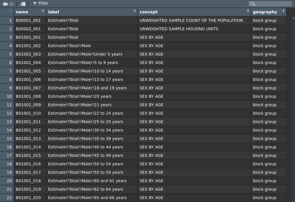
Figure 2.1: Variable viewer in RStudio
By browsing the table in this way, users can identify the appropriate variable IDs (found in the name column) that can be passed to the variables parameter in get_acs() or get_decennial(). Users may note that the raw variable IDs in the ACS, as consumed by the API, require a suffix of E or M. tidycensus does not require this suffix, as it will automatically return both the estimate and margin of error for a given requested variable. Additionally, if users desire an entire table of related variables from the ACS, the user should supply the characters prior to the underscore from a variable ID to the table parameter.
2.4 Data structure in tidycensus
Key to the design philosophy of tidycensus is its interpretation of tidy data. Following Wickham (2014), “tidy” data are defined as follows:
- Each observation forms a row;
- Each variable forms a column;
- Each observational unit forms a table.
By default, tidycensus returns a tibble of ACS or decennial Census data in “tidy” format. For decennial Census data, this will include four columns:
GEOID, representing the Census ID code that uniquely identifies the geographic unit;NAME, which represents a descriptive name of the unit;variable, which contains information on the Census variable name corresponding to that row;value, which contains the data values for each unit-variable combination. For ACS data, two columns replace thevaluecolumn:estimate, which represents the ACS estimate, andmoe, representing the margin of error around that estimate.
Given the terminology used by the Census Bureau to distinguish data, it is important to provide some clarifications of nomenclature here. Census or ACS variables, which are specific series of data available by enumeration unit, are interpreted in tidycensus as characteristics of those enumeration units. In turn, rows in datasets returned when output = "tidy", which is the default setting in the get_acs() and get_decennial() functions, represent data for unique unit-variable combinations. An example of this is illustrated below with income groups by state for the 2016 1-year American Community Survey.
hhinc <- get_acs(
  geography = "state",
  table = "B19001",
  survey = "acs1",
  year = 2016
)| GEOID | NAME | variable | estimate | moe |
|---|---|---|---|---|
| 01 | Alabama | B19001_001 | 1852518 | 12189 |
| 01 | Alabama | B19001_002 | 176641 | 6328 |
| 01 | Alabama | B19001_003 | 120590 | 5347 |
| 01 | Alabama | B19001_004 | 117332 | 5956 |
| 01 | Alabama | B19001_005 | 108912 | 5308 |
| 01 | Alabama | B19001_006 | 102080 | 4740 |
| 01 | Alabama | B19001_007 | 103366 | 5246 |
| 01 | Alabama | B19001_008 | 91011 | 4699 |
| 01 | Alabama | B19001_009 | 86996 | 4418 |
| 01 | Alabama | B19001_010 | 74864 | 4210 |
In this example, each row represents state-characteristic combinations, consistent with the tidy data model. Alternatively, if a user desires the variables spread across the columns of the dataset, the setting output = "wide" will enable this. For ACS data, estimates and margins of error for each ACS variable will be found in their own columns. For example:
hhinc_wide <- get_acs(
  geography = "state",
  table = "B19001",
  survey = "acs1",
  year = 2016,
  output = "wide"
)| GEOID | NAME | B19001_001E | B19001_001M | B19001_002E | B19001_002M | B19001_003E | B19001_003M | B19001_004E | B19001_004M | B19001_005E | B19001_005M | B19001_006E | B19001_006M | B19001_007E | B19001_007M | B19001_008E | B19001_008M | B19001_009E | B19001_009M | B19001_010E | B19001_010M | B19001_011E | B19001_011M | B19001_012E | B19001_012M | B19001_013E | B19001_013M | B19001_014E | B19001_014M | B19001_015E | B19001_015M | B19001_016E | B19001_016M | B19001_017E | B19001_017M |
|---|---|---|---|---|---|---|---|---|---|---|---|---|---|---|---|---|---|---|---|---|---|---|---|---|---|---|---|---|---|---|---|---|---|---|---|
| 28 | Mississippi | 1091245 | 8803 | 113124 | 4835 | 87136 | 5004 | 71206 | 4058 | 70160 | 4560 | 59619 | 4105 | 62688 | 4149 | 55973 | 4422 | 57215 | 4119 | 41870 | 3427 | 86198 | 4669 | 98865 | 5983 | 117664 | 5168 | 68367 | 4079 | 37809 | 2983 | 34786 | 3038 | 28565 | 2396 |
| 29 | Missouri | 2372190 | 10844 | 160615 | 6705 | 122649 | 4654 | 123789 | 5201 | 128270 | 5714 | 123224 | 4726 | 133429 | 5639 | 123373 | 4564 | 117476 | 5796 | 107254 | 4130 | 200473 | 6468 | 248099 | 6281 | 296437 | 7492 | 188700 | 6361 | 102034 | 4905 | 102670 | 4935 | 93698 | 4434 |
| 30 | Montana | 416125 | 4426 | 26734 | 2183 | 24786 | 2391 | 22330 | 2391 | 22193 | 2098 | 22568 | 2191 | 24449 | 2343 | 22135 | 2094 | 22241 | 1974 | 20513 | 1987 | 33707 | 2860 | 43775 | 3112 | 50902 | 2878 | 29940 | 2823 | 18585 | 1928 | 15669 | 1603 | 15598 | 1511 |
| 31 | Nebraska | 747562 | 4452 | 45794 | 3116 | 33266 | 2466 | 31084 | 2533 | 37602 | 2475 | 38037 | 3067 | 40412 | 2841 | 36761 | 2757 | 35558 | 2474 | 33429 | 2688 | 57950 | 3212 | 83173 | 4291 | 99028 | 4389 | 69003 | 3272 | 37347 | 2482 | 37665 | 2540 | 31453 | 2166 |
| 32 | Nevada | 1055158 | 6433 | 68507 | 4886 | 42720 | 3071 | 53143 | 3653 | 53188 | 3403 | 56693 | 3758 | 57215 | 3909 | 50798 | 4207 | 53783 | 3826 | 44637 | 3558 | 87876 | 4032 | 116975 | 4704 | 135242 | 4728 | 88474 | 4750 | 54275 | 3382 | 45943 | 3019 | 45689 | 3255 |
| 33 | New Hampshire | 520643 | 5191 | 20890 | 2566 | 15933 | 1908 | 18190 | 2315 | 18067 | 1841 | 21680 | 2292 | 22695 | 2067 | 21064 | 2112 | 17717 | 2340 | 21086 | 2454 | 39534 | 3108 | 57994 | 3587 | 75337 | 4214 | 56445 | 3069 | 33685 | 2445 | 41092 | 3028 | 39234 | 2925 |
| 34 | New Jersey | 3194519 | 10274 | 170029 | 6836 | 118862 | 5855 | 123335 | 6065 | 121889 | 4670 | 120881 | 5562 | 113762 | 5328 | 112003 | 5795 | 110312 | 6000 | 100527 | 4994 | 207103 | 6096 | 277719 | 8225 | 390127 | 9002 | 328144 | 8879 | 220764 | 7203 | 295764 | 7663 | 383298 | 7529 |
| 35 | New Mexico | 758364 | 6296 | 66983 | 4439 | 48930 | 3220 | 50025 | 4091 | 48054 | 3477 | 40353 | 3418 | 38164 | 2931 | 35107 | 2934 | 37564 | 2815 | 34581 | 2684 | 59437 | 3388 | 73011 | 3581 | 87486 | 4182 | 55708 | 3629 | 29307 | 2585 | 26732 | 2351 | 26922 | 2608 |
| 36 | New York | 7209054 | 17665 | 543763 | 12132 | 352029 | 9607 | 322683 | 7756 | 327051 | 8184 | 297201 | 8689 | 316465 | 9191 | 285531 | 8078 | 277776 | 8886 | 239908 | 8368 | 485826 | 10467 | 648930 | 12717 | 864777 | 14413 | 646586 | 12798 | 432309 | 11182 | 521545 | 11193 | 646674 | 9931 |
| 37 | North Carolina | 3882423 | 16063 | 282491 | 7816 | 228088 | 7916 | 209825 | 6844 | 212659 | 7095 | 206371 | 7190 | 215759 | 6349 | 190497 | 7507 | 199257 | 6269 | 170320 | 6503 | 318567 | 7932 | 395160 | 9069 | 468022 | 10041 | 288626 | 7339 | 160589 | 6395 | 166800 | 5286 | 169392 | 5628 |
The wide-form dataset includes GEOID and NAME columns, as in the tidy dataset, but is also characterized by estimate/margin of error pairs across the columns for each Census variable in the table.
2.4.1 Understanding GEOIDs
The GEOID column returned by default in tidycensus can be used to uniquely identify geographic units in a given dataset. For geographies within the core Census hierarchy (Census block through state, as discussed in Section 1.2), GEOIDs can be used to uniquely identify specific units as well as units’ parent geographies. Let’s take the example of households by Census block from the 2020 Census in Cimarron County, Oklahoma.
cimarron_blocks <- get_decennial(
  geography = "block",
  variables = "H1_001N",
  state = "OK",
  county = "Cimarron",
  year = 2020,
  sumfile = "pl"
)| GEOID | NAME | variable | value |
|---|---|---|---|
| 400259501001984 | Block 1984, Block Group 1, Census Tract 9501, Cimarron County, Oklahoma | H1_001N | 0 |
| 400259503001035 | Block 1035, Block Group 1, Census Tract 9503, Cimarron County, Oklahoma | H1_001N | 0 |
| 400259503001068 | Block 1068, Block Group 1, Census Tract 9503, Cimarron County, Oklahoma | H1_001N | 5 |
| 400259503001146 | Block 1146, Block Group 1, Census Tract 9503, Cimarron County, Oklahoma | H1_001N | 0 |
| 400259503001197 | Block 1197, Block Group 1, Census Tract 9503, Cimarron County, Oklahoma | H1_001N | 7 |
| 400259503001218 | Block 1218, Block Group 1, Census Tract 9503, Cimarron County, Oklahoma | H1_001N | 2 |
| 400259501001067 | Block 1067, Block Group 1, Census Tract 9501, Cimarron County, Oklahoma | H1_001N | 0 |
| 400259501001118 | Block 1118, Block Group 1, Census Tract 9501, Cimarron County, Oklahoma | H1_001N | 0 |
| 400259501001141 | Block 1141, Block Group 1, Census Tract 9501, Cimarron County, Oklahoma | H1_001N | 0 |
| 400259501001223 | Block 1223, Block Group 1, Census Tract 9501, Cimarron County, Oklahoma | H1_001N | 0 |
The mapping between the GEOID and NAME columns in the returned 2020 Census block data offers some insight into how GEOIDs work for geographies within the core Census hierarchy. Take the first block in the table, Block 1110, which has a GEOID of 400259503001110. The GEOID value breaks down as follows:
The first two digits, 40, correspond to the Federal Information Processing Series (FIPS) code for the state of Oklahoma. All states and US territories, along with other geographies at which the Census Bureau tabulates data, will have a FIPS code that can uniquely identify that geography.
Digits 3 through 5, 025, are representative of Cimarron County. These three digits will uniquely identify Cimarron County within Oklahoma. County codes are generally combined with their corresponding state codes to uniquely identify a county within the United States, as three-digit codes will be repeated across states. Cimarron County’s code in this example would be 40025.
The next six digits, 950300, represent the block’s Census tract. The tract name in the
NAMEcolumn is Census Tract 9503; the six-digit tract ID is right-padded with zeroes.The twelfth digit, 1, represents the parent block group of the Census block. As there are no more than nine block groups in any Census tract, the block group name will not exceed 9.
The last three digits, 110, represent the individual Census block, though these digits are combined with the parent block group digit to form the block’s name.
For geographies outside the core Census hierarchy, GEOIDs will uniquely identify geographic units but will only include IDs of parent geographies to the degree to which they nest within them. For example, a geography that nests within states but may cross county boundaries like school districts will include the state GEOID in its GEOID but unique digits after that. Geographies like core-based statistical areas that do not nest within states will have fully unique GEOIDs, independent of any other geographic level of aggregation such as states.
2.4.2 Renaming variable IDs
Census variables IDs can be cumbersome to type and remember in the course of an R session. As such, tidycensus has built-in tools to automatically rename the variable IDs if requested by a user. For example, let’s say that a user is requesting data on median household income (variable ID B19013_001) and median age (variable ID B01002_001). By passing a named vector to the variables parameter in get_acs() or get_decennial(), the functions will return the desired names rather than the Census variable IDs. Let’s examine this for counties in Georgia from the 2016-2020 five-year ACS.
ga <- get_acs(
  geography = "county",
  state = "Georgia",
  variables = c(medinc = "B19013_001",
                medage = "B01002_001"),
  year = 2020
)| GEOID | NAME | variable | estimate | moe |
|---|---|---|---|---|
| 13001 | Appling County, Georgia | medage | 39.9 | 1.7 |
| 13001 | Appling County, Georgia | medinc | 37924.0 | 4761.0 |
| 13003 | Atkinson County, Georgia | medage | 35.9 | 1.5 |
| 13003 | Atkinson County, Georgia | medinc | 35703.0 | 5493.0 |
| 13005 | Bacon County, Georgia | medage | 36.5 | 1.0 |
| 13005 | Bacon County, Georgia | medinc | 36692.0 | 3774.0 |
| 13007 | Baker County, Georgia | medage | 52.2 | 4.8 |
| 13007 | Baker County, Georgia | medinc | 34034.0 | 9879.0 |
| 13009 | Baldwin County, Georgia | medage | 35.8 | 0.5 |
| 13009 | Baldwin County, Georgia | medinc | 46250.0 | 4707.0 |
ACS variable IDs, which would be found in the variable column, are replaced by medage and medinc, as requested. When a wide-form dataset is requested, tidycensus will still append E and M to the specified column names, as illustrated below.
ga_wide <- get_acs(
  geography = "county",
  state = "Georgia",
  variables = c(medinc = "B19013_001",
                medage = "B01002_001"),
  output = "wide",
  year = 2020
)| GEOID | NAME | medincE | medincM | medageE | medageM |
|---|---|---|---|---|---|
| 13001 | Appling County, Georgia | 37924 | 4761 | 39.9 | 1.7 |
| 13003 | Atkinson County, Georgia | 35703 | 5493 | 35.9 | 1.5 |
| 13005 | Bacon County, Georgia | 36692 | 3774 | 36.5 | 1.0 |
| 13007 | Baker County, Georgia | 34034 | 9879 | 52.2 | 4.8 |
| 13011 | Banks County, Georgia | 50912 | 4278 | 41.5 | 1.1 |
| 13013 | Barrow County, Georgia | 62990 | 2562 | 36.0 | 0.3 |
| 13017 | Ben Hill County, Georgia | 32077 | 4008 | 39.5 | 1.4 |
| 13021 | Bibb County, Georgia | 41317 | 1220 | 36.3 | 0.3 |
| 13023 | Bleckley County, Georgia | 46992 | 6279 | 36.0 | 1.5 |
| 13027 | Brooks County, Georgia | 37516 | 4438 | 43.6 | 0.9 |
Median household income for each county is represented by medincE, for the estimate, and medincM, for the margin of error. At the time of this writing, custom variable names are only available for variables and not for table, as users will not always know the number of variables found in a table beforehand.
2.5 Other Census Bureau datasets in tidycensus
As mentioned earlier in this chapter, tidycensus does not grant access to all of the datasets available from the Census API; users should look at the censusapi package (Recht 2021) for that functionality. However, the Population Estimates and ACS Migration Flows APIs are accessible with the get_estimates() and get_flows() functions, respectively. This section includes brief examples of each.
2.5.1 Using get_estimates()
The Population Estimates Program, or PEP, provides yearly estimates of the US population and its components between decennial Censuses. It differs from the ACS in that it is not directly based on a dedicated survey, but rather projects forward data from the most recent decennial Census based on birth, death, and migration rates. In turn, estimates in the PEP will differ slightly from what you may see in data returned by get_acs(), as the estimates are produced using a different methodology.
One advantage of using the PEP to retrieve data is that allows you to access the indicators used to produce the intercensal population estimates. These indicators can be specified as variables direction in the get_estimates() function in tidycensus, or requested in bulk by using the product argument. The products available include "population", "components", "housing", and "characteristics". For example, we can request all components of change population estimates for 2019 for a specific county:
library(tidycensus)
library(tidyverse)

queens_components <- get_estimates(
  geography = "county",
  product = "components",
  state = "NY",
  county = "Queens",
  year = 2019
)| NAME | GEOID | variable | value |
|---|---|---|---|
| Queens County, New York | 36081 | BIRTHS | 27453.000000 |
| Queens County, New York | 36081 | DEATHS | 16380.000000 |
| Queens County, New York | 36081 | DOMESTICMIG | -41789.000000 |
| Queens County, New York | 36081 | INTERNATIONALMIG | 9883.000000 |
| Queens County, New York | 36081 | NATURALINC | 11073.000000 |
| Queens County, New York | 36081 | NETMIG | -31906.000000 |
| Queens County, New York | 36081 | RBIRTH | 12.124644 |
| Queens County, New York | 36081 | RDEATH | 7.234243 |
| Queens County, New York | 36081 | RDOMESTICMIG | -18.456152 |
| Queens County, New York | 36081 | RINTERNATIONALMIG | 4.364836 |
The returned variables include raw values for births and deaths (BIRTHS and DEATHS) during the previous 12 months, defined as mid-year 2018 (July 1) to mid-year 2019. Crude rates per 1000 people in Queens County are also available with RBIRTH and RDEATH. NATURALINC, the natural increase, then measures the number of births minus the number of deaths. Net domestic and international migration are also available as counts and rates, and the NETMIG variable accounts for the overall migration, domestic and international included. Alternatively, a single variable or vector of variables can be requested with the variable argument, and the output = "wide" argument can also be used to spread the variable names across the columns.
The product = "characteristics" argument also has some unique options. The argument breakdown lets users get breakdowns of population estimates for the US, states, and counties by "AGEGROUP", "RACE", "SEX", or "HISP" (Hispanic origin). If set to TRUE, the breakdown_labels argument will return informative labels for the population estimates. For example, to get population estimates by sex and Hispanic origin for metropolitan areas, we can use the following code:
louisiana_sex_hisp <- get_estimates(
  geography = "state",
  product = "characteristics",
  breakdown = c("SEX", "HISP"),
  breakdown_labels = TRUE,
  state = "LA",
  year = 2019
)| GEOID | NAME | value | SEX | HISP |
|---|---|---|---|---|
| 22 | Louisiana | 4648794 | Both sexes | Both Hispanic Origins |
| 22 | Louisiana | 4401822 | Both sexes | Non-Hispanic |
| 22 | Louisiana | 246972 | Both sexes | Hispanic |
| 22 | Louisiana | 2267050 | Male | Both Hispanic Origins |
| 22 | Louisiana | 2135979 | Male | Non-Hispanic |
| 22 | Louisiana | 131071 | Male | Hispanic |
| 22 | Louisiana | 2381744 | Female | Both Hispanic Origins |
| 22 | Louisiana | 2265843 | Female | Non-Hispanic |
| 22 | Louisiana | 115901 | Female | Hispanic |
The value column gives the estimate characterized by the population labels in the SEX and HISP columns. For example, the estimated population value in 2019 for Hispanic males in Louisiana was 131,071.
2.5.2 Using get_flows()
As of version 1.0, tidycensus also includes support for the ACS Migration Flows API. The flows API returns information on both in- and out-migration for states, counties, and metropolitan areas. By default, the function allows for analysis of in-migrants, emigrants, and net migration for a given geography using data from a given 5-year ACS sample. In the example below, we request migration data for Honolulu County, Hawaii. In-migration for world regions is available along with out-migration and net migration for US locations.
honolulu_migration <- get_flows(
  geography = "county",
  state = "HI",
  county = "Honolulu",
  year = 2019
)| GEOID1 | GEOID2 | FULL1_NAME | FULL2_NAME | variable | estimate | moe |
|---|---|---|---|---|---|---|
| 15003 | NA | Honolulu County, Hawaii | Africa | MOVEDIN | 152 | 156 |
| 15003 | NA | Honolulu County, Hawaii | Africa | MOVEDOUT | NA | NA |
| 15003 | NA | Honolulu County, Hawaii | Africa | MOVEDNET | NA | NA |
| 15003 | NA | Honolulu County, Hawaii | Asia | MOVEDIN | 7680 | 884 |
| 15003 | NA | Honolulu County, Hawaii | Asia | MOVEDOUT | NA | NA |
| 15003 | NA | Honolulu County, Hawaii | Asia | MOVEDNET | NA | NA |
| 15003 | NA | Honolulu County, Hawaii | Central America | MOVEDIN | 192 | 100 |
| 15003 | NA | Honolulu County, Hawaii | Central America | MOVEDOUT | NA | NA |
| 15003 | NA | Honolulu County, Hawaii | Central America | MOVEDNET | NA | NA |
| 15003 | NA | Honolulu County, Hawaii | Caribbean | MOVEDIN | 97 | 78 |
get_flows() also includes functionality for migration flow mapping; this advanced feature will be covered in Section 6.6.1.
2.6 Debugging tidycensus errors
At times, you may think that you’ve formatted your use of a tidycensus function correctly but the Census API doesn’t return the data you expected. Whenever possible, tidycensus carries through the error message from the Census API or translates common errors for the user. In the example below, a user has mis-typed the variable ID:
state_pop <- get_decennial(
  geography = "state",
  variables = "P01001",
  year = 2010
)
## Error : Your API call has errors. The API message returned is error: error: unknown variable 'P01001'.## Error in UseMethod("gather"): no applicable method for 'gather' applied to an object of class "character"The “unknown variable” error message from the Census API is carried through to the user. In other instances, users might request geographies that are not available in a given dataset:
cbsa_ohio <- get_acs(
  geography = "cbsa",
  variables = "DP02_0068P",
  state = "OH",
  year = 2019
)
## Error: Your API call has errors. The API message returned is error: unknown/unsupported geography heirarchy.The user above has attempted to get bachelor’s degree attainment by CBSA in Ohio from the ACS Data Profile. However, CBSA geographies are not available by state given that many CBSAs cross state boundaries. In response, the API returns an “unsupported geography hierarchy” error.
To assist with debugging errors, or more generally to help users understand how tidycensus functions are being translated to Census API calls, tidycensus offers a parameter show_call that when set to TRUE prints out the actual API call that tidycensus is making to the Census API.
cbsa_bachelors <- get_acs(
  geography = "cbsa",
  variables = "DP02_0068P",
  year = 2019,
  show_call = TRUE
)
## Getting data from the 2015-2019 5-year ACS## Using the ACS Data Profile## Census API call: https://api.census.gov/data/2019/acs/acs5/profile?get=DP02_0068PE%2CDP02_0068PM%2CNAME&for=metropolitan%20statistical%20area%2Fmicropolitan%20statistical%20area%3A%2AThe printed URL https://api.census.gov/data/2019/acs/acs5/profile?get=DP02_0068PE%2CDP02_0068PM%2CNAME&for=metropolitan%20statistical%20area%2Fmicropolitan%20statistical%20area%3A%2A can be copy-pasted into a web browser where users can see the raw JSON returned by the Census API and inspect the results.
[["DP02_0068PE","DP02_0068PM","NAME","metropolitan statistical area/micropolitan statistical area"],
["15.7","1.5","Big Stone Gap, VA Micro Area","13720"],
["31.6","1.0","Billings, MT Metro Area","13740"],
["27.9","0.7","Binghamton, NY Metro Area","13780"],
["31.4","0.4","Birmingham-Hoover, AL Metro Area","13820"],
["33.3","1.0","Bismarck, ND Metro Area","13900"],
["21.2","2.0","Blackfoot, ID Micro Area","13940"],
["35.2","1.1","Blacksburg-Christiansburg, VA Metro Area","13980"],
["44.8","1.1","Bloomington, IL Metro Area","14010"],
["40.8","1.2","Bloomington, IN Metro Area","14020"],
["24.9","1.0","Bloomsburg-Berwick, PA Metro Area","14100"],
...
A common use-case for show_call = TRUE is to understand what data is available from the API, especially if functions in tidycensus are returning NA in certain rows. If the raw API call itself contains missing values for given variables, this will confirm that the requested data are not available from the API at a given geography.
2.7 Exercises
Review the available geographies in tidycensus from the geography table in this chapter. Acquire data on median age (variable
B01002_001) for a geography we have not yet used.Use the
load_variables()function to find a variable that interests you that we haven’t used yet. Useget_acs()to fetch data from the 2016-2020 ACS for counties in the state where you live, where you have visited, or where you would like to visit.